Wavelet Toolbox

One-Dimensional Analysis Using the Command Line

This example involves a real-world signal -- electrical consumption measured over the course of 3 days. This signal is particularly interesting because of noise introduced when a defect developed in the monitoring equipment as the measurements were being made. Wavelet analysis effectively removes the noise.

Loading a Signal.   

1. From the MATLAB prompt, type:

   load leleccum; 
   

2. Set the variables. Type:

   s = leleccum(1:3920); 
   l_s = length(s);
   

Performing A Single-Level Wavelet Decomposition of a Signal.   

3. Perform a single-level decomposition of the signal using the db1 wavelet. Type:

   [cA1,cD1] = dwt(s,'db1');
   

This generates the coefficients of the level 1 approximation (cA1) and detail (cD1).

Constructing Approximations and Details from the Coefficients.   

4. To construct the level 1 approximation and detail (A1 and D1) from the coefficients cA1 and cD1, type:

   A1 = upcoef('a',cA1,'db1',1,l_s); 
   D1 = upcoef('d',cD1,'db1',1,l_s);
   

or

A1 = idwt(cA1,[],'db1',l_s); 
D1 = idwt([],cD1,'db1',l_s);

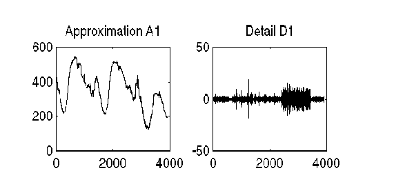
Displaying the Approximation and Detail.   

5. To display the results of the level-one decomposition, type:

   subplot(1,2,1); plot(A1); title('Approximation A1')
   subplot(1,2,2); plot(D1); title('Detail D1') 
   

Regenerating a Signal by Using the Inverse Wavelet Transform.   

6. To find the inverse transform, type:

   A0 = idwt(cA1,cD1,'db1',l_s);
   err = max(abs(s-A0))
   
   err = 
        2.2737e-013
   

Performing a Multilevel Wavelet Decomposition of a Signal.   

7. To perform a level 3 decomposition of the signal (again using the db1 wavelet), type:

   [C,L] = wavedec(s,3,'db1');
   

The coefficients of all the components of a third-level decomposition (that is, the third-level approximation and the first three levels of detail) are returned concatenated into one vector, C. Vector L gives the lengths of each component.

Extracting Approximation and Detail Coefficients.   

8. To extract the level 3 approximation coefficients from C, type:

   cA3 = appcoef(C,L,'db1',3);
   

9. To extract the levels 3, 2, and 1 detail coefficients from C, type:

   cD3 = detcoef(C,L,3); 
   cD2 = detcoef(C,L,2); 
   cD1 = detcoef(C,L,1);
   or
   [cD1,cD2,cD3] = detcoef(C,L,[1,2,3]);
   

Results are displayed in the figure below, which contains the signal s, the approximation coefficients at level 3 (cA3), and the details coefficients from level 3 to 1 (cD3, cD2 and cD1) from the top to the bottom.

Reconstructing the Level 3 Approximation.   

10. To reconstruct the level 3 approximation from C, type:

    A3 = wrcoef('a',C,L,'db1',3);
    

Reconstructing the Level 1, 2, and 3 Details.   

11. To reconstruct the details at levels 1, 2 and 3, from C, type:

    D1 = wrcoef('d',C,L,'db1',1);
    D2 = wrcoef('d',C,L,'db1',2);
    D3 = wrcoef('d',C,L,'db1',3);
    

Displaying the Results of a Multilevel Decomposition.   

12. To display the results of the level 3 decomposition, type:

    subplot(2,2,1); plot(A3); 
    title('Approximation A3')
    subplot(2,2,2); plot(D1); 
    title('Detail D1')
    subplot(2,2,3); plot(D2); 
    title('Detail D2')
    subplot(2,2,4); plot(D3); 
    title('Detail D3')
    
    
    

Reconstructing the Original Signal From the Level 3 Decomposition.   

13. To reconstruct the original signal from the wavelet decomposition structure, type:

    A0 = waverec(C,L,'db1');
    
    err = max(abs(s-A0))
    
    err = 
        4.5475e-013
    

Crude De-noising of a Signal.   

Using wavelets to remove noise from a signal requires identifying which component or components contain the noise, and then reconstructing the signal without those components.

In this example, we note that successive approximations become less and less noisy as more and more high-frequency information is filtered out of the signal.

The level 3 approximation, A3, is quite clean as a comparison between it and the original signal.

14. To compare the approximation to the original signal, type:

    subplot(2,1,1);plot(s);title('Original'); axis off
    subplot(2,1,2);plot(A3);title('Level 3 Approximation');
    axis off
    
    
    

Of course, in discarding all the high-frequency information, we've also lost many of the original signal's sharpest features.

Optimal de-noising requires a more subtle approach called thresholding. This involves discarding only the portion of the details that exceeds a certain limit.

Removing Noise by Thresholding.   

Let's look again at the details of our level 3 analysis.

15. To display the details D1, D2, and D3, type:

    subplot(3,1,1); plot(D1); title('Detail Level 1'); axis off
    subplot(3,1,2); plot(D2); title('Detail Level 2'); axis off
    subplot(3,1,3); plot(D3); title('Detail Level 3'); axis off
    
    
    

Most of the noise occurs in the latter part of the signal, where the details show their greatest activity. What if we limited the strength of the details by restricting their maximum values? This would have the effect of cutting back the noise while leaving the details unaffected through most of their durations. But there's a better way.

Note that cD1, cD2, and cD3 are just MATLAB vectors, so we could directly manipulate each vector, setting each element to some fraction of the vectors' peak or average value. Then we could reconstruct new detail signals D1, D2, and D3 from the thresholded coefficients.

16. To de-noise the signal, use the ddencmp command to calculate the default parameters and the wdencmp command to perform the actual de-noising, type:

    [thr,sorh,keepapp] = ddencmp('den','wv',s);
    clean = wdencmp('gbl',C,L,'db1',3,thr,sorh,keepapp);
    

Note that wdencmp uses the results of the decomposition (C and L) that we calculated in Step 7. We also specify that we used the db1 wavelet to perform the original analysis, and we specify the global thresholding option 'gbl'. See ddencmp and wdencmp in the reference pages for more information about the use of these commands.

17. To display both the original and de-noised signals, type:

    subplot(2,1,1); plot(s(2000:3920)); title('Original')
    subplot(2,1,2); plot(clean(2000:3920)); title('De-noised')
    
    
    

We've plotted here only the noisy latter part of the signal. Notice how we've removed the noise without compromising the sharp detail of the original signal. This is a strength of wavelet analysis.

While using command line functions to remove the noise from a signal can be cumbersome, the Wavelet Toolbox graphical interface tools include an easy-to-use de-noising feature that includes automatic thresholding.

More information on the de-noising process can be found in the following sections:

• Removing Noise From a Signal
• De-Noising
• One-Dimensional Variance Adaptive Thresholding of Wavelet Coefficients
• One-Dimensional Variance Adaptive Thresholding of Wavelet Coefficients

One-Dimensional Discrete Wavelet Analysis

One-Dimensional Analysis Using the Graphical Interface