| Spline Toolbox | |
NURBS and Other Rational Splines
A rational spline is, by definition, any function that is the ratio of two splines:
This requires w to be scalar-valued, but s is often chosen to be vector-valued. Further, it is desirable that w(x) be not zero for any x of interest.
Rational splines are popular because, in contrast to ordinary splines, they can be used to describe certain basic design shapes, like conic sections, exactly. For example,
circle = rsmak('circle');
provides a rational spline whose values on its basic interval trace out the unit circle, i.e., the circle of radius 1 with center at the origin, as the command
fnplt(circle), axis square
readily shows; have a look at the resulting plot, in Figure 1-13.
Figure 1-13: A Circle and an Ellipse, Both Given By a Rational Spline
It is easy to manipulate this circle to obtain related shapes. For example, the next commands stretch the circle into an ellipse, rotate the ellipse 45 degrees, and translate it by (1,1), and then plot it on top of the circle.
ellipse = fncmb(circle,[2 0;0 1]);
s45 = 1/sqrt(2);
rtellipse = fncmb(fncmb(ellipse, [s45 -s45;s45 s45]), [1;1] );
hold on, fnplt(rtellipse), hold off
As a further example, the `circle' just constructed is put together from four pieces. We highlight the first such piece, by the following commands:
quarter = fnbrk(fn2fm(circle,'rp'),1);
hold on, fnplt(quarter,3), hold off
In the first command, fn2fm is used to change forms, from one based on the B-form to one based on the ppform, and then fnbrk is used to extract the first piece, and this piece is then plotted on top of the circle in Figure 1-13, with linewidth 3 to make it stand out.
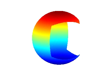
As a surface example, the command rsmak(`southcap') provides a 3-vector valued rational bicubic polynomial whose values on the unit square [-1 .. 1]^2 fill out a piece of the unit sphere. Adjoin to it five suitable rotates of it and you get the unit sphere exactly. For illustration, the following commands generate 2/3 of that sphere, as shown in Figure 1-14.
southcap = rsmak('southcap'); fnplt(southcap)
xpcap = fncmb(southcap,[0 0 -1;0 1 0;1 0 0]);
ypcap = fncmb(xpcap,[0 -1 0; 1 0 0; 0 0 1]);
northcap = fncmb(southcap,-1);
hold on, fnplt(xpcap), fnplt(ypcap), fnplt(northcap)
axis equal, shading interp, view(-115,10), axis off, hold off
Figure 1-14: Part of a Sphere Formed by Four Rotates of a Quartic Rational
Offhand, the two splines, s and w, in the rational spline r(x) = s(x)/w(x) need not at all be related to one another. They could even be of different forms. But, in the context of this toolbox, it is convenient to restrict them to be of the same form, and even of the same order and with the same breaks or knots. For, under that assumption, we can (and do) represent such a rational spline by the (vector-valued) spline function
whose values are vectors with one more entry than the values of the rational spline r. It is very easy to obtain r(x) from R(x). For example, if v is the value of R at x, then v(1:end-1)/v(end) is the value of r at x. If, in addition, dv is DR(x), then (dv(1:end-1)-dv(end)*v(1:end-1))/v(end) is Dr(x). More generally, by Leibniz' formula,
This shows that we can compute the derivatives of r inductively, using the derivatives of s and w (i.e., the derivatives of R) along with the derivatives of r of order less than j to compute the j-th derivative of r. There is a corresponding formula for partial and directional derivatives for multivariate rational splines.
Having chosen to represent the rational spline r = s/w in this way by the ordinary spline R = [s;w] makes it is easy to apply to a rational spline all the fn... commands in the Spline Toolbox, with the following exceptions. The integral of a rational spline need not be a rational spline, hence there is no way to extend fnint to rational splines. The derivative of a rational spline is again a rational spline but one of roughly twice the order. For that reason, fnder and fndir will not touch rational splines. Instead, there is the command fntlr for computing the value at a given x of all derivatives up to a given order of a given function. If that function is rational, the needed calculation is based on the considerations given in the preceding paragraph.
A special rational spline, called a NURBS, has become a standard tool in CAGD. A NURBS is, by definition, any rational spline for which both s and w are in B-form, with each coefficient for s containing explicitly the corresponding coefficient for w as a factor:
The normalized coefficients a(:,i) for the numerator spline are more readily used as control points than the unnormalized coefficients v(i)a(:,i). Nevertheless, this toolbox provides no special NURBS form, but only the more general rational spline, but in both B-form (called rBform internally) and in ppform (called rpform internally).
The rational spline circle used earlier is put together in rsmak by commands like the following.
x = [1 1 0 -1 -1 -1  0  1 1]; y = [0 1 1  1  0 -1 -1 -1 0];
s45 = 1/sqrt(2); w =[1 s45 1 s45 1 s45 1 s45 1];
circle = rsmak(augknt(0:4,3,2), [w.*x;w.*y;w]);
Note the appearance of the denominator spline as the last component. Also note how the coefficients of the denominator spline appear here explicitly as factors of the corresponding coefficients of the numerator spline. The normalized coefficient sequence [x;y] is very simple; it consists of the vertices and midpoints, in proper order, of the `unit square'. The resulting control polygon is tangent to the circle at the places where the four quadratic pieces that form the circle abut.
For a thorough discussion of NURBS, see [G. Farin, NURBS, 2nd ed., AKPeters Ltd, 1999] or [Les Piegl and Wayne Tiller, The NURBS Book, 2nd ed., Springer-Verlag, 1997].
| | Tensor Product Splines | Example: A Nonlinear ODE | |