Signal Processing Toolbox

lpc

Compute linear prediction filter coefficients.

Syntax

a = lpc(x,p)

Description

lpc determines the coefficients of a forward linear predictor by minimizing the prediction error in the least squares sense. It has applications in filter design and speech coding.

a = lpc(x,p) finds the coefficients of a pth-order linear predictor (FIR filter) that predicts the current value of the real-valued time series x based on past samples.

p is the order of the prediction filter polynomial, a = [1 a(2) ... a(p+1)]. If p is unspecified, lpc uses as a default p = length(x)-1. If x is a matrix containing a separate signal in each column, lpc returns a model estimate for each column in the rows of matrix a.

Examples

Estimate a data series using a third-order forward predictor, and compare to the original signal.

First, create the signal data as the output of an autoregressive process driven by white noise. Use the last 4096 samples of the AR process output to avoid start-up transients.

randn('state',0);
noise = randn(50000,1);  % Normalized white Gaussian noise
x = filter(1,[1 1/2 1/3 1/4],noise);
x = x(45904:50000);

Compute the predictor coefficients, estimated signal, prediction error, and autocorrelation sequence of the prediction error.

a = lpc(x,3);
est_x = filter([0 -a(2:end)],1,x);    % Estimated signal
e = x - est_x;                        % Prediction error
[acs,lags] = xcorr(e,'coeff');        % ACS of prediction error

The prediction error, e(n), can be viewed as the output of the prediction error filter A(z) shown below, where H(z) is the optimal linear predictor, x(n) is the input signal, and is the predicted signal.

Compare the predicted signal to the original signal.

plot(1:97,x(4001:4097),1:97,est_x(4001:4097),'--');
title('Original Signal vs. LPC Estimate');
xlabel('Sample Number'); ylabel('Amplitude'); grid;
legend('Original Signal','LPC Estimate')

Look at the autocorrelation of the prediction error.

plot(lags,acs); 
title('Autocorrelation of the Prediction Error');
xlabel('Lags'); ylabel('Normalized Value'); grid;

The prediction error is approximately white Gaussian noise, as expected for a third-order AR input process.

Algorithm

lpc uses the autocorrelation method of autoregressive (AR) modeling to find the filter coefficients. The generated filter might not model the process exactly even if the data sequence is truly an AR process of the correct order. This is because the autocorrelation method implicitly windows the data, that is, it assumes that signal samples beyond the length of x are 0.

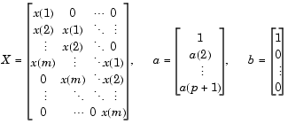
lpc computes the least squares solution to

where

and m is the length of x. Solving the least squares problem via the normal equations

leads to the Yule-Walker equations

where r = [r(1) r(2) ... r(p+1)] is an autocorrelation estimate for x computed using xcorr. The Yule-Walker equations are solved in O(p²) flops by the Levinson-Durbin algorithm (see levinson).

See Also

aryule	Compute an estimate of AR model parameters using the Yule-Walker method.
levinson	Compute the Levinson-Durbin recursion.
prony	Prony's method for time domain IIR filter design.
pyulear	Estimate the power spectral density using the Yule-Walker AR method.
stmcb	Compute a linear model using Steiglitz-McBride iteration.

References

[1] Jackson, L.B., Digital Filters and Signal Processing, Second Edition, Kluwer Academic Publishers, 1989. pp. 255-257.

lp2lp

lsf2poly