

| Partial Differential Equations Toolbox | |
Assemble boundary condition contributions.
[Q,G,H,R]=assemb(b,p,e)
[Q,G,H,R]=assemb(b,p,e,u0)
[Q,G,H,R]=assemb(b,p,e,u0,time)
[Q,G,H,R]=assemb(b,p,e,u0,time,sdl)
[Q,G,H,R]=assemb(b,p,e,time)
[Q,G,H,R]=assemb(b,p,e,time,sdl)
Description
[Q,G,H,R]=assemb(b,p,e)
assembles the matrices Q and H, and the vectors G and R. Q should be added to the system matrix and contains contributions from mixed boundary conditions. G should be added to the right-hand side and contains contributions from generalized Neumann and mixed boundary conditions. The equation H*u=R represents the Dirichlet type boundary conditions.
p, e, u0, time, and sdl have the same meaning as in assempde.
b
describes the boundary conditions of the PDE problem. b can be either a Boundary Condition matrix or the name of a Boundary M-file. The format of the Boundary Condition matrix is described below, and the format of the Boundary M-file is described in the entry on pdebound.
The toolbox treats the following boundary condition types:
 · (c
· (c u) + qu = g.
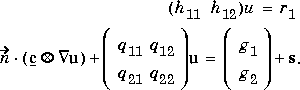
 . Let the number of variables in the system be N. Our general boundary condition is
hu = r
. Let the number of variables in the system be N. Our general boundary condition is
hu = r
By the notation  · (c
· (c  u) we mean the N-by-1 matrix with (i,1)-component

 is the angle of the normal vector of the boundary, pointing in the direction out from , the domain.
The Boundary Condition matrix is created internally in
is the angle of the normal vector of the boundary, pointing in the direction out from , the domain.
The Boundary Condition matrix is created internally in pdetool (actually a function called by pdetool) and then used from the function assemb for assembling the contributions from the boundary to the matrices Q, G, H, and R. The Boundary Condition matrix can also be saved onto a file as a boundary M-file for later use with the wbound function.
For each column in the Decomposed Geometry matrix there must be a corresponding column in the Boundary Condition matrix. The format of each column is according to the list below:
Row one contains the dimension N of the system.
Row two contains the number M of Dirichlet boundary conditions.
Row three to 3 + N2 - 1 contain the lengths for the strings representing  .The lengths are stored in column-wise order with respect to
  .
Row 3 + N2 to 3 + N2 +N- 1 contain the lengths for the strings representing g.
Row 3 + N2 + N to 3 + N2 + N + MN - 1 contain the lengths for the strings representing h. The lengths are stored in column-wise order with respect to h.
Row 3 + N2 + N + NM to 3 + N2 + N + MN + M - 1 contain the lengths for the strings representing r.
The following rows contain MATLAB text expressions representing the actual boundary condition functions. The text strings have the lengths according to above. The MATLAB text expressions are stored in column-wise order with respect to matrices h and
.
Row 3 + N2 to 3 + N2 +N- 1 contain the lengths for the strings representing g.
Row 3 + N2 + N to 3 + N2 + N + MN - 1 contain the lengths for the strings representing h. The lengths are stored in column-wise order with respect to h.
Row 3 + N2 + N + NM to 3 + N2 + N + MN + M - 1 contain the lengths for the strings representing r.
The following rows contain MATLAB text expressions representing the actual boundary condition functions. The text strings have the lengths according to above. The MATLAB text expressions are stored in column-wise order with respect to matrices h and  . There are no separation characters between the
strings. You can insert MATLAB expressions containing the following variables:
. There are no separation characters between the
strings. You can insert MATLAB expressions containing the following variables:
x and y
s, proportional to arc length. s is 0 at the start of the boundary segment and increases to 1 along the boundary segment in the direction indicated by the arrow.
nx and ny. If you need the tangential vector, it can be expressed using nx and ny since tx = -ny and ty = nx.
u (only if the input argument u has been specified)
t (only if the input argument time has been specified)
Examples
The following examples describe the format of the boundary condition matrix. For a boundary in a scalar PDE (N = 1) with Neumann boundary condition
(M = 0)
 · (cu) = -x2,
 the boundary condition would be represented by the column vector
[1 0 1 5 '0' '-x.^2']'
is stored in the column vector
[1 1 1 1 1 9For a system (N = 2) with mixed boundary conditions (M = 1)'0''0''1''x.^2-y.^2']'
2
1
lq11
lq21
lq12
lq22
lg1
lg2
lh11
lh12
lr1
q11 ...
q21 ...
q12 ...
q22 ...
g1 ...
g2 ...
h11 ...
h12 ...
r1 ...
Where
lq11, lq21, . . . denote lengths of the MATLAB text expressions, and q11, q21, . . . denote the actual expressions.
You can easily create your own examples by trying out pdetool. Enter boundary conditions by double-clicking on boundaries in boundary mode, and then export the Boundary Condition matrix to the MATLAB main workspace by selecting the Export Decomposed Geometry, Boundary Cond's . . . option from the Boundary menu.
| assema | assempde | |
 · (c
· (c  + h'µ.