Spline Toolbox

The B-form

A univariate spline f  is specified by its nondecreasing knot sequence t and by its B-spline coefficient sequence a; -- see the section on Tensor Product Splines for a discussion of multivariate splines. The coefficients may be d-vectors, usually 2-vectors or 3-vectors and required to be written as 1-column matrices, in which case f  is a curve in 2-space or 3-space and the coefficients are called the control points for the curve.

Roughly speaking, such a spline is piecewise-polynomial of a certain order and with breaks t(i). But knots are different from breaks in that they may be repeated, i.e., t need not be strictly increasing. The resulting knot multiplicities govern the smoothness of the spline across the knots, as detailed below.

With [d,n] = size(a), and n+k = length(t), the spline is of order k. This means that its polynomial pieces have degree < k. For example, a cubic spline is a spline of order 4 since it takes four coefficients to specify a cubic polynomial. These four items, t, a, n, and k, make up the B-form of the spline f.

This means, explicitly, that

with the ith B-spline of order k for the given knot sequence t, i.e., the B-spline with knots t(i), ..., t(i+k). The basic interval of this B-form is the interval [t(1)..t(n+k)]. It is the default interval over which a spline in B-form is plotted by the command fnplt. Note that a spline in B-form is zero outside its basic interval while, after conversion to ppform via fn2fm, this is usually not the case since, outside its basic interval, a piecewise-polynomial is defined by extension of its first or last polynomial piece.

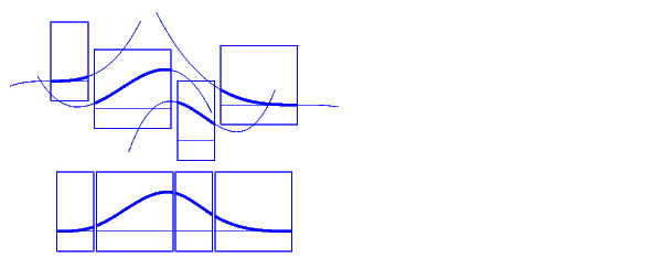
The building blocks for the B-form of a spline are the B-splines. The Figure 1-9 shows a picture of such a B-spline, the one with the knot sequence
[0 1.5 2.3 4 5], hence of order 4, together with the polynomials whose pieces make up the B-spline.The information for that picture could be generated by the command

bspline([0 1.5 2.3 4 5])

Figure 1-9: A B-Spline of Order 4, and the Four Cubic Polynomials from Which It Is Made

To summarize: The B-spline with knots is positive on the interval (t(i)..t(i+k)) and is zero outside that interval. It is piecewise-polynomial of order k with breaks at the sites t(i), ..., t(i+k). These knots may coincide, and the precise multiplicity governs the smoothness with which the two polynomial pieces join there. The rule is:

knot multiplicity + condition multiplicity = order

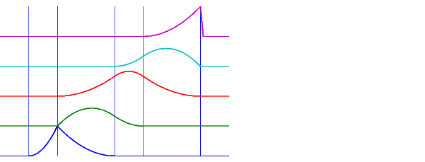
Figure 1-10: All Third-Order B-Splines for a Certain Knot Sequence with Various Knot Multiplicities

For example, for a B-spline of order 3, a simple knot would mean two smoothness conditions, i.e., continuity of function and first derivative, while a double knot would only leave one smoothness condition, i.e., just continuity, and a triple knot would leave no smoothness condition, i.e., even the function would be discontinuous.

Figure 1-10 shows a picture of all the third-order B-splines for a certain mystery knot sequence t. The breaks are indicated by vertical lines. For each break, try to determine its multiplicity in the knot sequence (it is 1,2,1,1,3), as well as its multiplicity as a knot in each of the B-splines. For example, the second break has multiplicity 2 but appears only with multiplicity 1 in the third B-spline and not at all, i.e., with multiplicity 0, in the last two B-splines. Note that only one of the B-splines shown has all its knots simple. It is the only one having three different nontrivial polynomial pieces. Note also that you can tell the knot-sequence multiplicity of a knot by the number of B-splines whose nonzero part begins or ends there. The picture is generated by the following MATLAB statements which use the command spcol from this toolbox to generate the function values of all these B-splines at a fine net x.

t=[0,1,1,3,4,6,6,6]; x=linspace(-1,7,81); 
c=spcol(t,3,x);[l,m]=size(c); 
c=c+ones(l,1)*[0:m-1]; 
axis([-1 7 0 m]); hold on 
for tt=t, plot([tt tt],[0 m],'-'), end 
plot(x,c,'linew',2), hold off, axis off

Further illustrated examples are provided by the demo spalldem.

The rule "knot multiplicity + condition multiplicity = order" has the following consequence for the process of choosing a knot sequence for the B-form of a spline approximant: Suppose the spline s is to be of order k, with basic interval [a . .b], and with interior breaks . Suppose, further, that, at , the spline is to satisfy smoothness conditions, i.e.,  

Then, the appropriate knot sequence t should contain the break exactly
times, i = 2, ..., l. In addition, it should contain the two endpoints, a and b, of the basic interval exactly k times. This last requirement can be relaxed, but has become standard. With this choice, there is exactly one way to write each spline s with the properties described as a weighted sum of the B-splines of order k with knots a segment of the knot sequence t. This is the reason for the B in B-spline: B-splines are, in Schoenberg's terminology, basic splines.

For example, if you want to generate the B-form of a cubic spline on the interval [1 . . 3], with interior breaks 1.5, 1.8, 2.6, and with two continuous derivatives, then the following would be the appropriate knot sequence:

t = [1, 1, 1, 1, 1.5, 1.8, 2.6, 3, 3, 3, 3];

This is supplied by augknt([1, 1.5, 1.8, 2.6, 3], 4). If you wanted, instead, to allow for a corner at 1.8, i.e., a possible jump in the first derivative there, you would triple the knot 1.8, i.e., use

t = [1, 1, 1, 1, 1.5, 1.8, 1.8, 1.8, 2.6, 3, 3, 3, 3];

and this is provided by the statement

t = augknt([1, 1.5, 1.8, 2.6, 3], 4, [1, 3, 1] );

The shorthand

is one of several ways to indicate that f  is a spline of order k with knot sequence t, i.e., a linear combination of the B-splines of order k for the knot sequence t.

A word of caution: The term B-spline has been expropriated by the CAGD community to mean what is called here a spline in B-form, with the unhappy result that, in any discussion between mathematicians/approximation theorists and people in CAGD, one now always has to check in what sense the term is being used.

Usually, a spline is constructed from some information, like function values and/or derivative values, or as the approximate solution of some ordinary differential equation. But it is also possible to make up a spline from scratch, by providing its knot sequence and its coefficient sequence to the command spmak.

For example, we might say

sp = spmak(1:10,3:8);

thus supplying the uniform knot sequence 1:10 and the coefficient sequence 3:8. Since there are 10 knots and 6 coefficients, the order must be 4(= 10 - 6), i.e., we get a cubic spline. The command

fnbrk(sp) 

prints out the constituent parts of the B-form of this cubic spline, as follows:

knots(1:n+k) 
   1 2 3 4 5 6 7 8 9 10 
coefficients(d,n) 
   3 4 5 6 7 8 
number n of coefficients 
   6 
order k 
   4 
dimension d of target 
   1

Further, fnbrk can be used to supply each of these parts separately.

But the point of the Spline Toolbox is that there shouldn't be any need for you to look up these details. You simply use sp as an argument to commands that evaluate, differentiate, integrate, convert, or plot the spline whose description is contained in sp.

As another simple example,

points = .95*[0 -1 0 1;1 0 -1 0]; 
sp = spmak(-4:8,[points points]);

provides a planar, quartic, spline curve whose middle part is a pretty good approximation to a circle, as the plot on the next page shows. It is generated by a subsequent

plot(points(1,:),points(2,:),'x'), hold on 
fnplt(sp,[0,4]), axis equal square, hold off

Insertion of additional control points (±.95,±.95)/ would make a visually perfect circle.

Here are more details. The spline curve generated has the form

, with [-4:8] the uniform knot sequence, and with its control points a(:,j) the sequence (0, ), (-, 0), (0, -), (, 0), (0, ) (-, 0), (0, -), (, 0) with = .95. Only the curve part between the parameter values 0 and 4 is actually plotted.

To get a feeling for how close to circular this part of the curve actually is, we compute its unsigned curvature. The curvature at the curve point of a space curve can be computed from the formula

in which norm{a} is the Euclidean length of the 3-vector a, and is the cross product of the two 3-vectors a and b, and and are the first and second derivative of the curve with respect to the parameter used. We treat our planar curve as a space curve in the (x,y)-plane, hence obtain the maximum and minimum of its curvature at 21 points as follows:

t = linspace(0,4,21);zt = zeros(size(t));
dsp = fnder(sp); dspt = fnval(dsp,t); ddspt = fnval(fnder(dsp),t);
kappa = abs(dspt(1,:).*ddspt(2,:)-dspt(2,:).*ddspt(1,:))./...
   (sum(dspt.^2)).^(3/2);
[min(kappa),max(kappa)] 
ans = 1.6747    1.8611

So, while the curvature is not quite constant, it is close to 1/radius of the circle, as we see from the next calculation:

1/norm(fnval(sp,0)) 
ans = 1.7864 

Figure 1-11: Spline Approximation to a Circle; Control Points Are Marked x

The following commands are available for spline work. There is spmak and fnbrk to make up a spline and take it apart again. Use fn2fm to convert from B-form to ppform. You can evaluate, differentiate, integrate, plot, or refine a spline with the aid of fnval, fnder, fndir, fnint, fnplt, and fnrfn.

There are five commands for generating knot sequences:

• augknt for providing boundary knots and also controlling the multiplicity of interior knots
• brk2knt for supplying a knot sequence with specified multiplicities
• aptknt for providing a knot sequence for a spline space of given order that is suitable for interpolation at given data sites
• optknt for providing an optimal knot sequence for interpolation at given sites
• newknt for a knot sequence perhaps more suitable for the function to be approximated

In addition, there is:

• aveknt to supply certain knot averages (the Greville sites) as recommended sites for interpolation
• chbpnt to supply such sites
• knt2brk and knt2mlt for extracting the breaks and/or their multiplicities from a given knot sequence

For display of a spline curve with given two-dimensional coefficient sequence and a uniform knot sequence, there is spcrv.

You can also write your own spline construction commands, in which case you will need to know the following. The construction of a spline satisfying some interpolation or approximation conditions usually requires a collocation matrix, i.e., the matrix that, in each row, contains the sequence of numbers

, i.e., the rth derivative at of the jth B-spline, for all j, for some r and some site . Such a matrix is provided by spcol. An optional argument allows for this matrix to be supplied by spcol in a space-saving spline-almost-block-diagonal-form or as a MATLAB sparse matrix. It can be fed to slvblk, a command for solving linear systems with almost-block-diagonal coefficient matrix. If you are interested in seeing how spcol and slvblk are used in this toolbox, have a look at the commands spapi, spap2, and spaps.

In addition, there are routines for constructing cubic splines:

csapi and csape provide the cubic spline interpolant at knots to given data, using the not-a-knot and various other end conditions, respectively. A parametric cubic spline curve through given points is provided by cscvn. The cubic smoothing spline is constructed in csaps.

The remaining commands involving the B-form are utilities, of no interest to the casual user.

The ppform

Tensor Product Splines