Real-Time Workshop User's Guide

Tutorial 4: A First Look at Generated Code

In this tutorial, you examine code generated from a from a simple model, to observe the effects of one of the many code optimization features available in the Real-Time Workshop.

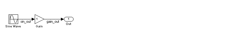
Figure 1-12 shows the source model.

Figure 1-12: example.mdl

Setting up the Model

First, create the model and set up basic Simulink and Real-Time Workshop parameters as follows:

1. Create a directory example_codegen, and make it your working directory.

   !mkdir example_codegen
   cd example_codegen
   

2. Create a new model and save it as example.mdl.
3. Add Sine Wave, Gain, and Out1 blocks to your model and connect them as shown in Figure 1-12. Label the signals as shown.
4. From the Simulation menu, choose Simulation Parameters. The Simulation Parameters dialog box opens.
5. Click the Solver tab and enter the following parameter values on the Solver page:

Solver options: set Type to Fixed-step. Select the ode5 (Dormand-Prince) solver algorithm.

Leave the other Solver page parameters set to their default values.

6. Click Apply.
7. Click the Workspace I/O tab and make sure all check boxes are deselected.
8. Click Apply.
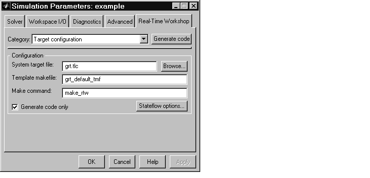
9. Click the Real-Time Workshop tab. Select Target configuration from the Category pull-down menu. Next, select the Generate code only option. This option causes the Real-Time Workshop to generate code without invoking make to compile and link the code. This option is convenient for this exercise, as we are only interested in looking at the generated code. Note that the Build button caption changes to Generate code.

Also, make sure that the generic real-time (GRT) target is selected. The page should appear as below.

10. Click Apply.
11. Save the model.

Generating Code Without Buffer Optimization

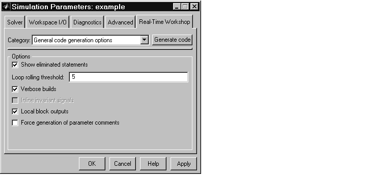
When the block I/O optimization feature is enabled, the Real-Time Workshop uses local storage for block outputs wherever possible. We now disable this option to see what the generated code looks like:

1. From the Simulation menu, choose Simulation Parameters. The Simulation Parameters dialog box opens.
2. Click the Advanced tab. Select the Signal storage reuse option and select the Off radio button, as shown below.
   
   
3. Click Apply.
4. Click the Real-Time Workshop tab and select the Target configuration category. Then click the Generate code button.
5. Because the Generate code only option was selected, the Real-Time Workshop does not invoke your make utility. The code generation process ends with the message

### Successful completion of Real-Time Workshop build procedure for model: example

6. The generated code is in the build directory, example_grt_rtw. The file example_grt_rtw\example.c contains the output computation for the model. Open this file into the MATLAB editor.

edit example_grt_rtw\example.c

7. In example.c, find the function MdlOutputs.

The generated C code consists of procedures that implement the algorithms defined by your Simulink block diagram. Your target's execution engine executes the procedures as time moves forward. The modules that implement the execution engine and other capabilities are referred to collectively as the run-time interface modules.

In our example, the generated MdlOutputs function implements the actual algorithm for multiplying a sine wave by a gain. The MdlOutputs function computes the model's block outputs. The run-time interface must call MdlOutputs at every time step.

With buffer optimizations turned off, MdlOutputs assigns buffers to each block input and output. These buffers (rtB.sin_out, rtB.gain_out) are members of a global data structure, rtB. The code is shown below.

void MdlOutputs(int_T tid)
{
  /* Sin Block: <Root>/Sine Wave */
  rtB.sin_out = rtP.Sine_Wave_Amp *
    sin(rtP.Sine_Wave_Freq * ssGetT(rtS) + rtP.Sine_Wave_Phase);
  /* Gain Block: <Root>/Gain */
  rtB.gain_out = rtB.sin_out * rtP.Gain_Gain;
  /* Outport Block: <Root>/Out1 */
  rtY.Out1 = rtB.gain_out;
}

We now turn buffer optimization on and observe how it improves the code.

Generating Code with Buffer Optimization

Enable buffer optimization and re-generate the code as follows:

1. From the Simulation menu, choose Simulation Parameters. The Simulation Parameters dialog box opens.
2. Click the Advanced tab. Select the Signal storage reuse option and select the On radio button.
3. Click Apply.
4. Click the Real-Time Workshop tab. Select General code generation options from the Category pull-down menu.

5. Make sure that the Local block outputs option is both enabled and selected, as shown above.
6. Click Apply and select the Target Configuration category again.
7. Click the Generate code button.
8. As before, the Real-Time Workshop generates code in the example_grt_rtw directory. Note that the previously-generated code is overwritten.
9. Edit example_grt_rtw/example.c, and examine the function MdlOutputs.

With buffer optimization enabled, the code in MdlOutputs reuses rtb_temp0, a temporary buffer with local scope, rather than assigning global buffers to each input and output.

void MdlOutputs(int_T tid)
{
  /* local block i/o variables */
  real_T rtb_temp0;
  /* Sin Block: <Root>/Sine Wave */
  rtb_temp0 = rtP.Sine_Wave_Amp *
    sin(rtP.Sine_Wave_Freq * ssGetT(rtS) + rtP.Sine_Wave_Phase);
  /* Gain Block: <Root>/Gain */
  rtb_temp0 *= rtP.Gain_Gain;
  /* Outport Block: <Root>/Out1 */
  rtY.Out1 = rtb_temp0;
}

This code is more efficient in terms of memory usage. The efficiency improvement gained by enabling Local block outputs would be more significant in a large model with many signals.

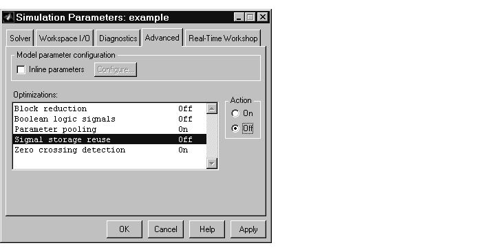
Note that, by default, Local block outputs is enabled. Chapter 3, Code Generation and the Build Process contains details on this and other code generation options.

For further information on the structure and execution of model.c files, refer to Chapter 6, Program Architecture.

Tutorial 3: Code Validation

Where to Find Information in This Manual