Optimization Toolbox

Quadratic Programming Solution

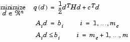
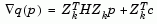
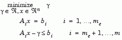
At each major iteration of the SQP method a QP problem is solved of the form where refers to the ith row of the m-by-n matrix .

(2-30)

The method used in the Optimization Toolbox is an active set strategy (also known as a projection method) similar to that of Gill et al., described in [18] and [17]. It has been modified for both Linear Programming (LP) and Quadratic Programming (QP) problems.

The solution procedure involves two phases: the first phase involves the calculation of a feasible point (if one exists), the second phase involves the generation of an iterative sequence of feasible points that converge to the solution. In this method an active set is maintained, , which is an estimate of the active constraints (i.e., which are on the constraint boundaries) at the solution point. Virtually all QP algorithms are active set methods. This point is emphasized because there exist many different methods that are very similar in structure but that are described in widely different terms.

is updated at each iteration, k, and this is used to form a basis for a search direction . Equality constraints always remain in the active set, . The notation for the variable, , is used here to distinguish it from in the major iterations of the SQP method. The search direction, , is calculated and minimizes the objective function while remaining on any active constraint boundaries. The feasible subspace for is formed from a basis, whose columns are orthogonal to the estimate of the active set (i.e., ). Thus a search direction, which is formed from a linear summation of any combination of the columns of , is guaranteed to remain on the boundaries of the active constraints.

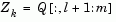
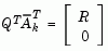
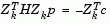
The matrix is formed from the last m-l columns of the QR decomposition of the matrix

, where l is the number of active constraints and l < m. That is, is given by

(2-31)

where

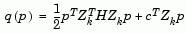
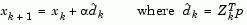
Having found , a new search direction is sought that minimizes where is in the null space of the active constraints, that is, is a linear combination of the columns of : for some vector p.

Then if we view our quadratic as a function of p, by substituting for , we have

(2-32)

Differentiating this with respect to p yields

(2-33)

is referred to as the projected gradient of the quadratic function because it is the gradient projected in the subspace defined by . The term is called the projected Hessian. Assuming the Hessian matrix H is positive definite (which is the case in this implementation of SQP), then the minimum of the function q(p) in the subspace defined by occurs when , which is the solution of the system of linear equations

(2-34)

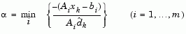
A step is then taken of the form

(2-35)

At each iteration, because of the quadratic nature of the objective function, there are only two choices of step length . A step of unity along is the exact step to the minimum of the function restricted to the null space of . If such a step can be taken, without violation of the constraints, then this is the solution to QP (Eq. 2.31). Otherwise, the step along to the nearest constraint is less than unity and a new constraint is included in the active set at the next iterate. The distance to the constraint boundaries in any direction is given by

(2-36)

which is defined for constraints not in the active set, and where the direction is towards the constraint boundary, i.e., .

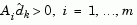When n independent constraints are included in the active set, without location of the minimum, Lagrange multipliers, are calculated that satisfy the nonsingular set of linear equations

(2-37)

If all elements of are positive, is the optimal solution of QP (Eq. 2.31). However, if any component of is negative, and it does not correspond to an equality constraint, then the corresponding element is deleted from the active set and a new iterate is sought.

Initialization

The algorithm requires a feasible point to start. If the current point from the SQP method is not feasible, then a point can be found by solving the linear programming problem

(2-38)

The notation indicates the ith row of the matrix A. A feasible point (if one exists) to Eq. 2.38 can be found by setting x to a value that satisfies the equality constraints. This can be achieved by solving an under- or over-determined set of linear equations formed from the set of equality constraints. If there is a solution to this problem, then the slack variable is set to the maximum inequality constraint at this point.

The above QP algorithm is modified for LP problems by setting the search direction to the steepest descent direction at each iteration where is the gradient of the objective function (equal to the coefficients of the linear objective function).

(2-39)

If a feasible point is found using the above LP method, the main QP phase is entered. The search direction is initialized with a search direction found from solving the set of linear equations

(2-40)

where is the gradient of the objective function at the current iterate (i.e., ).

If a feasible solution is not found for the QP problem, the direction of search for the main SQP routine is taken as one that minimizes .

Updating the Hessian Matrix

Line Search and Merit Function