smpcsim (Model Predictive Control Toolbox)

Simulates closed-loop systems with saturation constraints on the manipulated variables using models in the MPC mod format. Can also be used for open-loop simulations.

Syntax

yp = smpcsim(pmod,imod,Ks,tend,r) 
[yp,u,ym] = smpcsim(pmod,imod,Ks,tend,r,usat,... 
    Kest,z,d,w,wu)

Description

smpcsim provides a convenient way to simulate the performance of the type of system shown in the above diagram. The required input variables are as follows:

pmod
Is a model in the MPC mod format that is to represent the plant.

imod
Is a model in the MPC mod format that is to be used for state estimation in the controller. In general, it can be different from pmod if you wish to simulate the effect of plant/controller model mismatch. Note, however, that imod should be the same as that used to calculate Ks.

Ks
Is the MPC controller gain matrix, usually calculated using the function smpccon.

If you set Ks to an empty matrix, smpcsim will do an open-loop simulation. Then the inputs to the plant will be r (which must be set to the vector of manipulated variables in this case), d, w, and wu. The measurement noise input, z, will be ignored.

tend
Is the desired duration of the simulation (in time units).

r
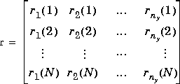
Is normally a setpoint matrix consisting of N rows and ny columns, where ny is the number of output variables, y:

where ri(k) is the setpoint for output j at time t = kT, and T is the sampling period (as specified by the minfo vector in the mod format of pmod and imod). If tend > NT, the setpoints vary for the first N periods in the simulation, as specified by r, and are then held constant at the values given in the last row of r for the remainder of the simulation.

In many simulations one wants the setpoints to be constant for the entire time, in which case r need only contain a single row of ny values.

If you set r=[ ], the default is a row of ny zeros.

For open-loop simulations, r specifies the manipulated variables and must contain nu columns.

The following input variables are optional. In general, setting one of them equal to an empty matrix causes smpcsim to use the default value, which is given in the description.

usat
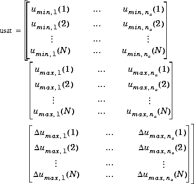
Is a matrix giving the saturation limits on the manipulated variables. Its format is as follows:

Note that it contains three matrices of N rows. N may be different than that for the setpoint matrix, r, but the idea is the same: the saturation limits will vary for the first N sampling periods of the simulation, then be held constant at the values given in the last row of usat for the remaining periods (if any).

The first matrix specifies the lower bounds on the nu manipulated variables. For example, umin,j(k) is the lower bound for manipulated variable j at time t = kT in the simulation. If umin,j(k) = -inf, manipulated variable j will have no lower bound at t = kT.

The second matrix gives the upper bounds on the manipulated variables. If umax,j(k) = inf, manipulated variable j will have no upper bound at t = kT.

The lower and upper bounds may be either positive or negative (or zero) as long as umin,j(k)

umax,j(k).

The third matrix gives the limits on the rate of change of the manipulated variables. In other words, smpcsim will force|uj(k) - uj(k - 1)|

umax,j(k). The limits on the rate of change must be nonnegative.

The default is no saturation constraints, i.e., all the umin values will be set to -inf, and all the umax and

umax values will be set to inf.

Note:
Saturation constraints are enforced by simply "clipping" the manipulated variable moves so that they satisfy all constraints. This is a nonoptimal solution that, in general, will differ from the results you would get using the ulim variable in scmpc.

Kest
Is the estimator gain matrix. The default is the DMC estimator. See smpcest for more details.

z
Is measurement noise that will be added to the outputs (see above diagram). The format is the same as for r. The default is a row of ny zeros.

d
Is a matrix of measured disturbances (see above diagram). The format is the same as for r, except that the number of columns is nd rather than ny. The default is a row of nd zeros.

w
Is a matrix of unmeasured disturbances (see above diagram). The format is the same as for r, except that the number of columns is nw rather than ny. The default is a row of nw zeros.I

wu
Is a matrix of unmeasured disturbances that are added to the manipulated variables (see above diagram). The format is the same as for r, except that the number of columns is nu rather than ny. The default is a row of nu zeros.

Note:
You may use a different number of rows in the matrices r, usat, z, d, w and wu, should that be appropriate for your simulation.

The calculated outputs are as follows (all but yp are optional):

yp
Is a matrix containing M rows and ny columns, where
M = max(fix(tend=T) + 1, 2). The first row will contain the initial condition, and row k - 1 will give the values of the plant outputs, y (see above diagram), at time t = kT.

u
Is a matrix containing the same number of rows as yp and nu columns. The time corresponding to each row is the same as for yp. The elements in each row are the values of the manipulated variables, u (see above diagram).

Note:
The u values are those coming from the controller before the addition of the unmeasured disturbance, wu.

ym
Is a matrix of the same structure as yp, containing the values of the predicted output from the state estimator in the controller. These will, in general, differ from those in yp if imodpmod and/or there are unmeasured disturbances. The prediction includes the effect of the most recent measurement, i.e., it is.

Examples
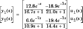
Consider the linear system:

The following statements build the model and calculate the MPC controller gain:

g11=poly2tfd(12.8,[16.7 1],0,1);
g21=poly2tfd(6.6,[10.9 1],0,7);
g12=poly2tfd(-18.9,[21.0 1],0,3);
g22=poly2tfd(-19.4,[14.4 1],0,3);
delt=3; ny=2;
imod=tfd2mod(delt,ny,g11,g21,g12,g22);
pmod=imod;
P=6; M=2;
ywt=[ ]; uwt=[1 1];
Ks=smpccon(imod,ywt,uwt,M,P);

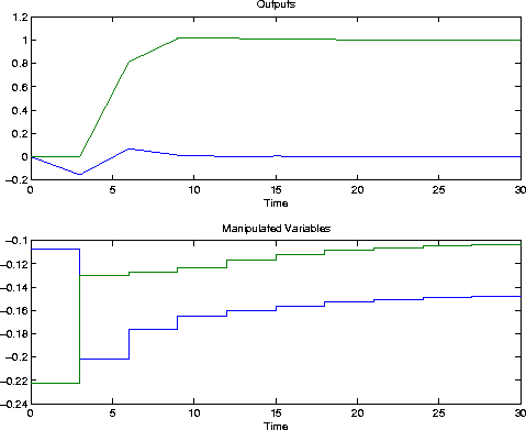
Simulate and plot the closed-loop performance for a unit step in the setpoint for y₂, occurring at t = 0.

tend=30; r=[0 1]; 
[y,u]=smpcsim(pmod,imod,Ks,tend,r); 
plotall(y,u,delt),pause

Try a pulse change in the disturbance that adds to u1:

r=[ ]; usat=[ ]; Kest=[ ]; z=[ ]; d=[ ]; w=[ ]; 
wu=[ 1 0; 0 0]; 
[y,u]=smpcsim(pmod,imod,Ks,tend,r,usat,Kest,z,d,w,wu);
plotall(y,u,delt),pause

For the same disturbance as in the previous case, limit the rates of change of both manipulated variables.

usat=[-inf -inf inf inf 0.1 0.05];
[y,u]=smpcsim(pmod,imod,Ks,tend,r,usat,Kest,z,d,w,wu);
plotall(y,u,delt),pause

Restrictions

Initial conditions of zero are used for all states in imod and pmod. This simulates the condition where all variables represent a deviation from a steady-state initial condition.
The first nu + nd columns of the D matrices in pmod and imod must be zero. In other words, neither u nor d may have an immediate effect on the outputs.

See Also
plotall, ploteach, scmpc, smpccl, smpccon, smpcest

smpcgain, smpcpole ss2mod