Linear Filtering and Filter Design (Image Processing Toolbox)

Image Processing Toolbox

Convolution

In MATLAB, linear filtering of images is implemented through two-dimensional convolution. In convolution, the value of an output pixel is computed by multiplying elements of two matrices and summing the results. One of these matrices represents the image itself, while the other matrix is the filter. For example, a filter might be

k = [4 -3  1
     4  6  2]

This filter representation is known as a convolution kernel. The MATLAB function conv2 implements image filtering by applying your convolution kernel to an image matrix. conv2 takes as arguments an input image and a filter, and returns an output image. For example, in this call, k is the convolution kernel, A is the input image, and B is the output image.

B = conv2(A,k);

conv2 produces the output image by performing these steps:

Rotate the convolution kernel 180 degrees to produce a computational molecule.
Determine the center pixel of the computational molecule.
Apply the computational molecule to each pixel in the input image.

Each of these steps is explained below.

Rotating the Convolution Kernel

In two-dimensional convolution, the computations are performed using a computational molecule. This is simply the convolution kernel rotated 180 degrees, as in this call.

h = rot90(k,2);

h = 

     2  6  4
     1 -3  4

Determining the Center Pixel

To apply the computational molecule, you must first determine the center pixel. The center pixel is defined as floor((size(h)+1)/2). For example, in a 5-by-5 molecule, the center pixel is (3,3). The molecule h shown above is 2-by-3, so the center pixel is (1,2).

Applying the Computational Molecule

The value of any given pixel in B is determined by applying the computational molecule h to the corresponding pixel in A. You can visualize this by overlaying h on A, with the center pixel of h over the pixel of interest in A. You then multiply each element of h by the corresponding pixel in A, and sum the results.

For example, to determine the value of the pixel (4,6) in B, overlay h on A, with the center pixel of h covering the pixel (4,6) in A. The center pixel is circled in Figure 6-1.

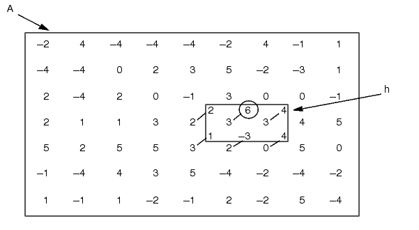
Figure 6-1: Overlaying the Computational Molecule for Convolution

Now, look at the six pixels covered by h. For each of these pixels, multiply the value of the pixel by the value in h. Sum the results, and place this sum in B(4,6).

B(4,6) = 2*2 + 3*6 + 3*4 + 3*1 + 2*-3 + 0*4 = 31

Perform this procedure for each pixel in A to determine the value of each corresponding pixel in B.

Linear Filtering Padding of Borders