Signal Processing Toolbox

Kaiser Window

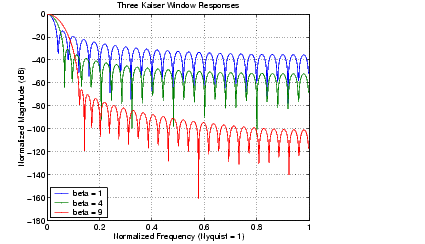
The Kaiser window is an approximation to the prolate-spheroidal window, for which the ratio of the mainlobe energy to the sidelobe energy is maximized. For a Kaiser window of a particular length, the parameter  controls the sidelobe height. For a given , the sidelobe height is fixed with respect to window length. The statement kaiser(n,beta) computes a length n Kaiser window with parameter beta.

Examples of Kaiser windows with length 50 and various values for the beta parameter are

n = 50;
w1 = kaiser(n,1);
w2 = kaiser(n,4);
w3 = kaiser(n,9);
[W1,f] = freqz(w1/sum(w1),1,512,2);
[W2,f] = freqz(w2/sum(w2),1,512,2);
[W3,f] = freqz(w3/sum(w3),1,512,2);
plot(f,20*log10(abs([W1 W2 W3]))); grid;
legend('beta = 1','beta = 4','beta = 9',3)
title('Three Kaiser Window Responses')
xlabel('Normalized Frequency (Nyquist = 1)')
ylabel('Normalized Magnitude (dB)')

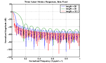
As increases, the sidelobe height decreases and the mainlobe width increases. To see how the sidelobe height stays the same for a fixed parameter as the length is varied, try

w1 = kaiser(50,4);
w2 = kaiser(20,4);
w3 = kaiser(101,4);
[W1,f] = freqz(w1/sum(w1),1,512,2);
[W2,f] = freqz(w2/sum(w2),1,512,2);
[W3,f] = freqz(w3/sum(w3),1,512,2);
plot(f,20*log10(abs([W1 W2 W3]))); grid;
legend('length = 50','length = 20','length = 101')
title('Three Kaiser Window Responses, Beta Fixed')
xlabel('Normalized Frequency (Nyquist = 1)')
ylabel('Normalized Magnitude (dB)')

Kaiser Windows in FIR Design

There are two design formulas that can help you design FIR filters to meet a set of filter specifications using a Kaiser window. To achieve a sidelobe height of - dB, the beta parameter is

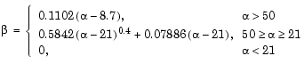
For a transition width of rad/s, use the length

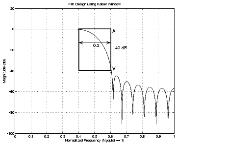
Filters designed using these heuristics will meet the specifications approximately, but you should verify this. To design a lowpass filter with cutoff frequency  rad/s, transition width  rad/s, and 40 dB of attenuation in the stopband, try

[n,wn,beta] = kaiserord([0.4 0.6]*pi,[1 0],[0.01 0.01],2*pi);
h = fir1(n,wn,kaiser(n+1,beta),'noscale');

The kaiserord function estimates the filter order, cutoff frequency, and Kaiser window beta parameter needed to meet a given set of frequency domain specifications.

The ripple in the passband is roughly the same as the ripple in the stopband. As you can see from the frequency response, this filter nearly meets the specifications.

[H,f] = freqz(h,1,512,2);
plot(f,20*log10(abs(H))), grid

For details on kaiserord, see the description in Chapter 7, "Function Reference.

Generalized Cosine Windows

Chebyshev Window