| Power System Blockset | |
Compute the state-space model of a linear electrical circuit
Synopsis
You must call circ2ss with a minimum of seven input arguments:
[A,B,C,D,states,x0,x0sw,rlsw,u,x,y,freq,Asw,Bsw,Csw,Dsw,Hlin]=
circ2ss(rlc,switches,source,line_dist,yout,y_type,unit)
You can also specify additional arguments. To use options, the number of input arguments must be 12, 13, 14 or 16:
[A,B,C,D,states,x0,x0sw,rlsw,u,x,y,freq,Asw,Bsw,Csw,Dsw,Hlin] =

circ2ss(rlc,switches,source,line_dist,yout,y_type,unit,net_arg1
,net_arg2,net_arg3,...

netsim_flag,fid_outfile,freq_sys,ref_node,vary_name,vary_val)
Description
Computes the state-space model of a linear electrical circuit expressed as
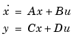
where x is the vector of state-space variables (inductor currents and capacitor voltages), u is the vector of voltage and current inputs, and y is the vector of voltage and current outputs.
When you build a circuit from the Power System Blockset icons of the powerlib library, circ2ss is automatically called by power2sys. circ2ss has also been made available as a stand-alone function for expert users. This allows you to generate state-space models without using the Power System Blockset graphical user interface and to access options that are not available through powerlib. For example, you can specify transformers and mutual inductances with more than three windings.
The linear circuit may contain any combination of voltage and current sources, RLC branches, multiwinding transformers, mutually coupled inductances and switches. The state variables are inductor currents and capacitor voltages.
The state-space representation (matrices A,B,C,D and vector x0) computed by circ2ss can then be used in a Simulink system, via a State-Space block, to perform simulation of the electrical circuit (see Example section below). Nonlinear elements (mechanical or electronic switches, transformer saturation, machines, distributed parameter lines, etc.) can be connected to the linear circuit.
These Simulink models are interfaced with the linear circuit through voltage outputs and current inputs of the state-space model. You can find the models of the nonlinear elements provided with the Power System Blockset in the Powerlib_models library (see the Advanced Topics chapter).
Input Arguments
The number of input arguments must be 7, 12, 13, 14 or 16. Arguments 8 to 16 are optional. The first seven arguments that must be specified are:
rlc: Branch matrix specifying the network topology as well as the resistance R, inductance L, and capacitance C values. See format below.switches: Switch matrix. Specify an empty variable if no switches are used. See format below.source: Source matrix specifying the parameters of the electrical voltage and current sources. Specify an empty variable if no sources are used. See format below. line_dist: Distributed parameter line matrix. Specify an empty variable if no distributed lines are used. See format below.yout: String matrix of output expressions. See format below.y_type: Integer vector indicating output types (zero for voltage output, one for current output).unit: String specifying the units to be used for R, L, and C values in the rlc matrix. If unit='OHM', R L C values are specified in ohms  at the fundamental frequency specified by
 freq_sys (default value is 60 Hz). If unit= 'OMU', R L C values are specified in ohms (), millihenries (mH), and microfarads (µF).The last nine arguments are optional. The first three are used to pass arguments from the power2sys function. Hereafter, we describe only the arguments to be specified when circ2ss is used as a stand-alone function:
net_arg1, net_arg2, net_arg3: Used to pass arguments from power2sys. Specify empty variables [] for each of these variables. netsim_flag: Integer controlling the messages displayed during the execution of circ2ss. Default value is zero. If netsim_flag =0, the version number, number of states, inputs, outputs and modes are displayed. Output values are displayed in polar form for each source frequency.
If netsim_flag=1, only version number, number of states, inputs, and outputs are displayed.
If netsim_flag=2, no message is displayed during execution.
fid_outfile: File identifier of the circ2ss output file containing parameter values, node numbers, steady-state outputs, and special messages. Default value is zero.freq_sys: Fundamental frequency (Hz) considered for specification of XL and XC reactances if unit is set to 'OHM'. Default value is 60 Hz.ref_node: Reference node number used for ground of pi transmission lines. If -1 is specified, the user will be prompted to specify a node number.vary_name: String matrix containing the symbolic variable names used in output expressions. These variables must be defined in your MATLAB workspace.vary_val: Vector containing the values of the variable names specified in vary_name. Output Arguments
A,B,C,D: State-space matrices of the linear circuit with all switches open.nstates, nstates) B (nstates, ninput) C (noutput, nstates) D (noutput, ninput) where nstates is the number of state variables, ninput is the number of inputs, and noutput is the number of outputs.states: String matrix containing the names of the state variables. Each string has the following format:Inductor currents: Il_bxx_nzz1_zz2
Capacitor voltages: Uc_bxx_nzz1_zz2
where:
xx
zz1= first node number of the branch
zz2 = second node number of the branch
The last lines of the states matrix, which are followed by an asterisk, indicate inductor currents and capacitor voltages that are not considered as state variables. This situation arises when inductor currents or capacitor voltages are not independent (inductors forming a cutset or capacitors forming a loop). The currents and voltages followed by an asterisk can be expressed as a linear combination of the other state variables:
x0: Column vector of initial values of state variables considering the open or closed status of switches.x0sw: Vector of initial values of switch currents.rlsw: Matrix (nswitch,2) containing the R and L values of series switch impedances in ohms () and henries (H). nswitch is the number of switches in the circuit.u,x,y: Matrices u(ninput,nfreq), x(nstates,nfreq) and y(noutput,nfreq) containing the steady-state complex values of inputs, states and outputs. nfreq is the length of the freq vector. Each column corresponds to a different source frequency as specified by the next argument freq.freq: Column vector containing the source frequencies ordered by increasing frequencies.Asw,Bsw,Csw,Dsw: State-space matrices of the circuit including the closed switches. Each closed switch with an internal inductance adds one extra state to the circuit.Hlin: Three-dimensional array (nfreq, noutput, ninput) of the nfreq complex transfer impedance matrices of the linear system corresponding to each frequency of the freq vector.Format of the RLC Input Matrix
Nobr is assigned by the user.Each line of the RLC matrix must be specified according to the following format:
[node1, node2, type, R, L, C, Nobr] for RLC branch or line branch
[node1, node2, type, R, L, C, Nobr] for transformer magnetizing branch
[node1, node2, type, R, L, U, Nobr] for Transformer winding
[node1, node2, type, R, L, U, Nobr] for mutual inductances
node1: First node number of the branch. The node number must be positive or zero. Decimal node numbers are allowed. node2: Second node number of the branch. The node number must be positive or zero. Decimal node numbers are allowed. type: Integer indicating the type of connection of RLC elements, or the transmission line length (negative value).type=0: Series RLC element
type=1: Parallel RLC element
type=2: Transformer winding
type=3: Coupled (mutual) winding
If type is negative value: transmission line modeled by a PI section. See details below.
For a mutual inductor or a transformer having N windings, N+1 consecutive lines must be specified in RLC matrix:
type=2 or type=3; (one line per winding). Each line specifies R/L/U or R/Xl/Xc where [R/L, R/Xl = winding resistance and leakage reactance for a transformer or winding resistance and self reactance for mutually coupled windings. U is the nominal voltage of transformer winding (specify 0 if type =3).
type=1 for the magnetizing branch of a transformer (parallel Rm/Lm or Rm/Xm) or one line with type=0 for a mutual impedance (series Rm/Lm or Rm/Xm).
For a transformer magnetizing branch or a mutual impedance, the first node number is an internal node located behind the leakage reactance of the first winding. The second node number must be the same as the second node number of the first winding.
To model a saturable transformer, you must use a nonlinear inductance instead of the linear inductance simulating the reactive losses. Set the Lm/Xm value to zero (no linear inductance) and use the Transfosat block with proper flux-current characteristics.
This block can be found in the Powerlib_models library. This block must be connected to the linear part of the system (State-Space block or S-function) between a voltage output (voltage across the magnetizing branch) and a current input (current source injected into the transformer internal node). See the example given at the end of the circ2ss documentation.
If type is a negative value: length (km) of a transmission line simulated by a PI section. For a transmission line, the R/L/C or R/Xl/Xc values must be specified in (/km) or (, mH, or µF per km):
R: Branch resistance ().Xl: Branch inductive reactance ( at freq_sys) or transformer winding leakage reactance ( at freq_sys).L: Branch inductance (mH).Xc: Branch capacitive reactance ( at freq_sys) (The negative sign of Xc is optional).C: Capacitance (µF).U: Nominal voltage of transformer winding. Same units Volts or kV must be used for each winding. For a mutual inductance (type=3), this value must be set to zero.Zero values for R, L or Xl, C or Xc in a series or parallel branch indicate that the corresponding element does not exist.
The following restrictions apply for transformer winding R-L values. Null values are not allowed for secondary impedances if some transformer secondaries form loops (such as in a three-phase delta connection). Specify a very low value for R or L or both (e.g., 1e-6 p.u. based on rated voltage and power) to simulate a quasi-ideal transformer. The resistive and inductive parts of the magnetizing branch can be set to infinite (no losses; specify Xm=Rm=inf).
Format of the SOURCE Input Matrix
freq_sys.Each line of the source matrix must be specified according to the following format:
[ node1, node2, type, amp, phase, freq, model ]
node1, node2: Node numbers corresponding to the source terminalsnode1 is the positive terminal. Current source:node1 to node2 inside the source.type: Integer indicating the type of source: 0 for voltage source; 1 for current source.amp: Amplitude of the AC or DC voltage or current (V or A).phase: Phase of the AC voltage or current (degree).freq: Frequency (Hz) of the generated voltage or current. Default value is 60 Hz. For a DC voltage or current source specify phase=0 and freq=0. amp can be set to a negative value. The generated signals are: amp*sin(2*pi*freq*t+phase) for AC, amp for DC.model: Integer specifying the type of nonlinear element modeled by the current source (saturable inductance, thyristor, switch...). Used by power2sys only.Order in Which Sources Must Be Specified
The functions which compute the state-space representation of a system expect the sources to be in a certain order. This order must be respected in order to obtain correct results. You must be particularly careful if the system contains any switches. The following list gives the proper ordering of sources:
Refer to the Example section below for an example illustrating proper ordering of sources for a system containing nonlinear elements.
Format of the SWITCHES Input Matrix
Switches are nonlinear elements simulating mechanical or electronic devices such as circuit breakers, diodes, or thyristors. As other nonlinear elements, they are simulated by current sources driven by the voltage appearing across their terminals. Therefore, they cannot have a null impedance. They are simulated as ideal switches in series with a series R-L circuit. Various models of switches (circuit breaker, ideal switch, and power electronic devices) are available in the Powerlib_models library. They must be interconnected to the linear part of the system through appropriate voltage outputs and current inputs.
The switch parameters must be specified in a line of the switches matrix in seven different columns according to the following format:
[ node1, node2, status, R, L/Xl, no_I , no_U ]
node1, node2: Node numbers corresponding to the switch terminals.status: Code indicating the initial status of the switch at t=0.0= open; 1= closedR: Resistance of the switch when closed ().L/Xl: Inductance of the switch when closed (mH) or inductive reactance ( at freq_sys). Note: For these last two fields, the same units as those specified for the rlc matrix must be used. Either can be set to zero, but not both.
The next two fields specify the current input number and the voltage output number to be used for interconnecting the switch model to the state-space block. The output number corresponding to the voltage across a particular switch must be the same as the input number corresponding to the current from the same switch (see Example section below):
no_I: Current input number coming from the output of the switch model.no_U: Voltage output number driving the input of the switch model.Format of the LINE_DIST Matrix
The distributed parameter line model contains two parts:
Each row of the line_dist matrix is used to specify a distributed parameter transmission line. The number of columns of line_dist depends on the number of phases of the transmission line.
For an nphase line, the first (4+3*nhase+nphase^2) columns are used. For example, for a three-phase line, 22 columns are used:
[nphase, no_I, no_U, length, L/Xl, Zc, Rm, speed, Ti]
nphase: Number of phases of the transmission line.no_I: Input number in the source matrix corresponding to the first current source Is_1 of the line model. Each line model uses 2*nphase current sources specified in the source matrix as follows:no_U: Output number of the state-space corresponding to the first voltage output Vs_1 feeding the line model. Each line model uses 2*nphase voltage outputs in the source matrix as follows:length: Length of the line (km)Zc: Vector of the nphase modal characteristic impedances ()Rm: Vector of the nphase modal series resistances (/km)speed: Vector of the nphase modal propagation speeds (km/s)Ti: Transformation matrix from mode to phase currents such that Iphase=Ti.Imod. The nphase*nphase matrix must be given in vector format [col_1, col_2,... col_nphase].Format of the YOUT Matrix
The desired outputs are specified by a string matrix yout. Each line of the yout matrix must be an algebraic expression containing a linear combination of states and state derivatives specified according to the following format:
Uc_bn: Capacitor voltage of branch #n.Il_bn: Inductor current of branch #n.dUc_bn, dIl_bn: Derivative of Uc_bn or Il_bn.Un, In: Source voltage or current specified by line #n of the source matrix.U_nx1_x2: Voltage between nodes x1 and x2.I_bn: Current in branch #n. For a parallel RLC branch, I_bn corresponds to the total current IR+IL+IC.I_bn_nx: Current flowing into node x of a pi transmission line specified by line #n of the rlc matrix. This current includes the series inductive branch current and the capacitive shunt current.Each output expression is built from voltage and current variable names defined above, their derivatives, constants, other variable names, parenthesis and operators (+-*/^) in order to form a valid MATLAB expression. For example,
yout =char(['R1*I_b1+Uc_b3-L2*dIl_b2','U_n10_20','I2+3*I_b5']);
If variable names are used (R1 and L2 in the above example), their names and values must be specified by the two input arguments vary_name and vary_val.
Sign Conventions for Voltages and Currents
I_bn Il_bn, In: Branch current, inductor current of branch #n or current of source #n is oriented from node1 to node2.
I_bn_nxCurrent at one end (node x) of a pi transmission line. If x = node1, the current is entering the line. If x = node2, the current is leaving the line.:
Uc_bn, Un : Voltage across capacitor or source voltage (Unode1 - Unode2)
U_nx1_x2Voltage between nodes x1 and x2 = Ux1 - Ux2. Voltage of node x1 with respect to node x2.:
Order in Which Outputs Must Be Specified
The functions that compute the state-space representation of a system expect the outputs to be in a certain order. This order must be respected in order to obtain correct results. You must be particularly careful if the system contains any switches. The following list gives the proper ordering of outputs:
Refer to the Example section below for an example illustrating proper ordering of outputs for a system containing nonlinear elements.
Example
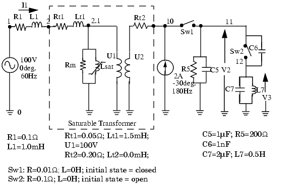
The following circuit consists of two sources (one voltage source and one current source), two series RLC branches (R1-L1 and C6), two parallel RLC branches (R5-C5 and L7-C7), one saturable transformer, and two switches (Sw1 and Sw2). Sw1 is initially closed whereas Sw2 is initially open. Three measurement outputs are specified (I1,V2, and V3). This circuit has seven nodes numbered 0, 1, 2, 2.1, 10, 11, and 12. Node 0 is used for the ground. Node 2.1 is the internal node of the transformer where the magnetization branch is connected.
You can use the circ2ss function to find the state-space model of the linear part of the circuit. The nonlinear elements Sw1, Sw2, and Lsat must be modeled separately by means of current sources driven by the voltage appearing across their terminals. Therefore you must foresee three additional currents sources and three additional voltage outputs for interfacing the nonlinear elements to the linear circuit.
You will obtain the state-space model of the circuit by entering the following commands in a MATLAB script file. The example is available in the psbcirc2ss.m file. Notice that an output text file containing information on the system is requested in the call to circ2ss.
unit='OMU'; % Units = Ohms, mH and uF

rlc=[
%N1 N2  typeR    L   C(uF)/U(V)
1   2   0   0.1  1   0   %R1 L1
2   0   2   0.05 1.5 100 %transfo Wind.#1
10  0   2   0.20 0   200 %transfo Wind.#2
2.1 0   1   1000 0   0   %transfo mag. branch
11  0   1   200  0   1   %R5 C5
11  12  0   0    0   1e-3%C6
12  0   1   0    500 2   %L7 C7
];

source=[
%N1 N2  typeU/I  phasefreq
10  11  1   0    0   0   %Sw1
11  12  1   0    0   0   %Sw2
2.1 0   1   0    0   0   %Saturation
1   0   0   100  0   60  %Voltage source
0   10  1   2    -30 180 %Current source
];

switches=[
%N1 N2  statusR(ohm)L(mH)I#U#
10  11  1   0.01 0   1   1   %Sw1
11  12  0   0.1  0   2   2   %Sw2
];

%outputs
%
% Both switches have Lon=0, so their voltages must be the first
outputs,
% immediatly followed by their currents (in the same order as the
voltages).
% The voltage across all nonlinear models which don't have L=0
follow (in
% this case the saturable transformer's magnetizing inductor).
The measure-
% ments which you request follow, in any order.
%
y_u1='U_n10_11';%U_Sw1= Voltage across Sw1
y_u2='U_n11_12';%U_Sw2= Voltage across Sw2
y_i3='I1';  %I1= Switch current Sw1
y_i4='I2';  %I2= Switch current Sw2
y_u5='U_n2.1_0';%U_sat= Voltage across saturable reactor
y_i6='I_b1';%I1 measurement
y_u7='U_n11_0';%V2 measurement
y_u8='U_n12_0';%V3 measurement

yout=char(y_u1,y_u2,y_i3,y_i4,y_u5,y_i6,y_u7,y_u8);% outputs
y_type=[0,0,1,1,0,1,0,0];%output types; 0=voltage 1=current

% Open file that will contain circ2ss output information
fid=fopen('psbcirc2ss.net','w');

[A,B,C,D,states,x0,x0sw,rlsw,u,x,y,freq,Asw,Bsw,Csw,Dsw,Hlin]=.
..

circ2ss(rlc,switches,source,[],yout,y_type,unit,[],[],[],0,fid)
;
While circ2ss is executing the following messages are displayed:
Computing state-space representation of linear electrical circuit
(V2.0)...
(4 states ; 5 inputs ; 7 outputs)

Oscillatory modes and damping factors:
F=159.115Hz zeta=4.80381e-08

Steady state outputs @ F=0 Hz :
y_u1= 0Volts
y_u2= 0Volts
y_i3= 0Amperes
y_i4= 0Amperes
y_u5= 0Volts
y_i6= 0Amperes
y_u7= 0Volts
y_u8= 0Volts
Steady state outputs @ F=60 Hz :
y_u1 = 0.009999 Volts < 3.168 deg.
y_u2 = 199.4 Volts < -1.148 deg.
y_i3 = 0.9999 Amperes < 3.168 deg.
y_i4 = 0 Amperes < 0 deg.
y_u5 = 99.81 Volts < -1.144 deg.
y_i6 = 2.099 Amperes < 2.963 deg.
y_u7 = 199.4 Volts < -1.148 deg.
y_u8 = 0.01652 Volts < 178.9 deg.

Steady state outputs @ F=180 Hz :
y_u1 = 0.00117 Volts < 65.23 deg.
y_u2 = 22.78 Volts < 52.47 deg.
y_i3 = 0.117 Amperes < 65.23 deg.
y_i4 = 0 Amperes < 0 deg.
y_u5 = 11.4 Volts < 53.48 deg.
y_i6 = 4.027 Amperes < 146.5 deg.
y_u7 = 22.83 Volts < 52.47 deg.
y_u8 = 0.0522 Volts < 52.47 deg.
The names of the state variables are returned in the states string matrix:
states
states =
Il_b2_n2_2.1
Uc_b5_n11_0
Uc_b6_n11_12
Il_b7_n12_0
Il_b1_n1_2*
Uc_b7_n12_0*
Although this circuit contains a total of six inductors and capacitors, there are only four state variables. The names of the state variables are given by the first four lines of the states matrix. The last two lines are followed by an asterisk indicating that these two variables are a linear combination of the state variables. The dependencies can be viewed in the output file psbcirc2ss.net:
The following capacitor voltages are dependant:
Uc_b7_n12_0 =  + Uc_b5_n11_0  - Uc_b6_n11_12
The following inductor currents are dependant:
Il_b1_n1_2 =  + Il_b2_n2_0
The A,B,C,D matrices contain the state-space model of the circuit without nonlinear elements (all switches open). The x0 vector contains the initial state values considering the switch Sw1 closed. The Asw, Bsw, Csw, and Dsw matrices contain the state-space model of the circuit considering the closed switch Sw1. The x0sw vector contains the initial current in the closed switch.
A
A =
    -4.0006e+05000
    0   -49950   -499.25
    0   -4992.50 4.9925e+05
    0   2   -2   0

Asw
Asw =
    -80.999-199.9900
    4.9947e+05-5244.70 -499.25
    4.9922e+05-5242.104.9925e+05
    0   2   -2   0
The system source frequencies are returned in the freq vector:
freq
freq =
     0    60   180
The corresponding steady-state complex outputs are returned in the (6-by-3) y matrix where each column corresponds to a different source frequency.
For example, you can obtain the magnitude of the six voltage and current outputs at 60 Hz as follows:
abs(y(:,2))
ans =
    0.0099987
    199.42
    0.99987
    0
    99.808
    2.0993
    199.41
    0.016519
The initial values of the four state variables are returned in the x0 vector. You must use this vector in the State-Space block to start the simulation in steady-state.
x0

x0 =
    2.3302
    14.111
    14.07
    3.1391e-05
The initial values of switch currents are returned in x0sw. To start the simulation in steady-state you must use these values as initial currents for the nonlinear model simulating the switches.
x0sw

x0sw =
    0.16155
    0
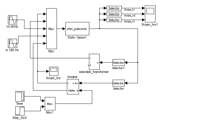
The Simulink model of the circuit is shown on the figure below and is available in the psbcirc2ss_slk.mdl file. The linear part of the circuit is simulated by the sfun_psbcontc S-function. Appropriate inputs and outputs are used to connect the switch and saturable reactance models to the linear system. Notice that the status of each switch is fed back from the breaker block to the S-function, after the inputs mentioned earlier. You can find the Breaker and Transfosat blocks in the Powerlib_models library containing all the nonlinear models used by the blockset. As the breaker model is vectorized, a single block is used to simulate the two switches Sw1 and Sw2.
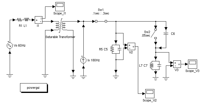
If you had used the powerlib library to build your circuit, the same Simulink system would have been generated automatically by the power2sys function. The powerlib version of this system is also available in the psbcirc2ss_psb.mdl file and is shown below.
Figure 5-1: psbcirc2ss_slk.mdl Example diagram
Figure 5-2: psbcirc2ss_psb.mdl Example Diagram
See Also
power2sys
| | Power System Commands | power2sys | |