Asynchronous Machine (Power System Blockset)

Model the dynamics of a three-phase asynchronous machine

Library

Machines

Description

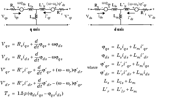
The Asynchronous Machine block operates in either generating or motoring mode. The mode of operation is dictated by the sign of the mechanical torque (positive for motoring, negative for generating). The electrical part of the machine is represented by a fourth-order state-space model and the mechanical part by a second-order system. All electrical variables and parameters are referred to the stator. This is indicated by the prime signs (') in the machine equations given below. All stator and rotor quantities are in the arbitrary two-axis reference frame (qd frame). The subscripts used are defined as follows:

d: d axis quantity

q: q axis quantity

r: rotor quantity

s: stator quantity

l: leakage inductance

m: magnetizing inductance

Electrical System

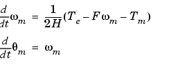
Mechanical System

The Asynchronous Machine block parameters are defined as follows (all quantities referred to the stator):

R_s, L_ls: stator resistance and leakage inductance

R'_r, L'_lr: rotor resistance and leakage inductance

L_m: magnetizing inductance

L_s, L'_r: total stator and rotor inductances

V_qs, i_qs: q axis stator voltage and current

V'_qr, i'_qr: q axis rotor voltage and current

V_ds, i_ds: d axis stator voltage and current

V'_dr, i'_dr: d axis rotor voltage and current

_qs, _ds: stator q and d axis fluxes

'_qr, '_dr: rotor q and d axis fluxes

_m: angular velocity of the rotor

_m: rotor angular position

p: number of pole pairs

_r: electrical angular velocity (_m x p)

_r: electrical rotor angular position (_m x p)

T_e: electromagnetic torque

T_m: shaft mechanical torque

J: combined rotor and load inertia coefficient (set to infinite to simulate locked rotor)

H: combined rotor and load inertia constant (set to infinite to simulate locked rotor)

F: combined rotor and load viscous friction coefficient

Parameters and Dialog Boxes

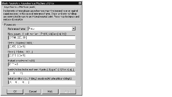
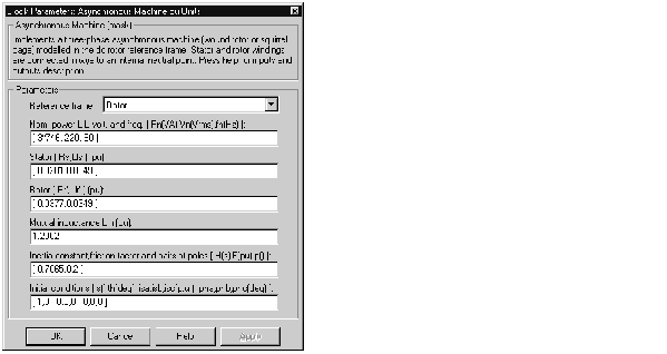
In the powerlib library you can choose between two Asynchronous Machine blocks to specify the electrical and mechanical parameters of the model.

S.I. Units Dialog Box

Reference Frame

Specifies the reference frame that is used to convert input voltages (abc reference frame) to the dq reference frame and output currents (dq reference frame) to the abc reference frame. You can choose between the following reference frame transformations:

Rotor (Park transformation)

Stationary (Clarke or transformation)

Synchronous

The following relationships describe the abc to qd reference frame transformations applied to the Asynchronous Machine block's input voltages.

In the above equations,

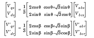is the angular position of the reference frame, while

is the difference between the position of the reference frame and the position (electrical) of the rotor. Since the machine windings are connected in a three-wire wye configuration, there is no homopolar (zero) component. This also justifies the fact that two line-to-line input voltages are used instead of three line-to-neutral voltages. The following relationships describe the qd to abc reference frame transformations applied to the Asynchronous Machine block's output currents.

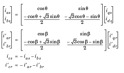The following table shows the values taken by

and

in each reference frame (

_e is the position of the synchronously rotating reference frame).


Reference Frame
Rotor	_r	0
Stationary	0	-_r
Synchronous	_e	_e - _r

The choice of reference frame will affect the waveforms of all dq variables. It will also affect the simulation speed and in certain cases the accuracy of the results. The following guidelines are suggested in [1]:

Use the stationary reference frame if the stator voltages are either unbalanced or discontinuous and the rotor voltages are balanced (or zero)

Use the rotor reference frame if the rotor voltages are either unbalanced or discontinuous and the stator voltages are balanced

Use either the stationary or synchronous reference frames if all voltages are balanced and continuous

Nominal: The nominal apparent power Pn (VA), rms line-to-line voltage Vn (V), and frequency fn (Hz).
Stator: The stator resistance Rs () and leakage inductance Lls (H).
Rotor: The rotor resistance Rr' () and leakage inductance Llr' (H), both referred to the stator.
Magnetizing inductance: The magnetizing inductance Lm (H).
Mechanical: The combined machine and load inertia coefficient J (kg.m²), combined viscous friction coefficient F (N.m.s), and pole pairs p.
Initial conditions: The initial slip s, electrical angle e (deg), stator currents magnitudes (A) and phase angles (deg). Can all be computed by the load flow utility in the Powergui block.

Per Unit (p.u.) Dialog Box

Reference frame: Specifies the reference frame that is used to convert input voltages (abc reference frame) to the dq reference frame and output currents (dq reference frame) to the abc reference frame. See the previous dialog box description for more detail.
Nominal: The nominal apparent power Pn (VA), rms line-to-line voltage Vn (V), and frequency fn (Hz).
Stator, Rotor, Mutual Inductance, Mechanical parameters: The same electrical and mechanical parameters as in the S.I. units dialog box, expressed in p.u., except inertia constant H, which is expressed in s.
Initial conditions: The same initial conditions as in the S.I. Units dialog box, except that current magnitudes are in p.u.

Note This block simulates exactly the same way as the asynchronous machine model; the only difference is the way of entering the parameter units.

Inputs and Outputs

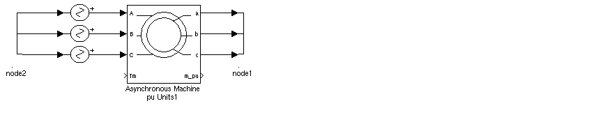
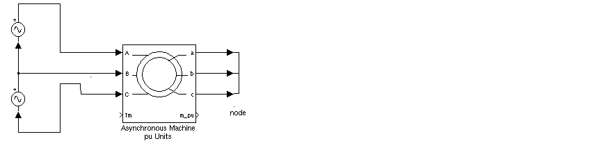
The electrical inputs of the block are the three electrical connections of the stator while the electrical outputs are the three electrical connections of the rotor. Note that the neutral connections of the stator and rotor windings are not available; three-wire Y connections are assumed. The rotor's connections should normally be short-circuited or connected to an external circuit, for example, external resistors or a power converter.

You must be careful when you connect ideal sources to the machine's stator. If you choose to supply the stator via a three-phase Y-connected infinite voltage source, you must use three sources connected in Y.

However, if you choose to simulate a delta source connection, you must only use two sources connected in series.

The Simulink input of the block is the mechanical torque at the machine's shaft. This input must be positive in the motoring mode and negative in the generating mode.

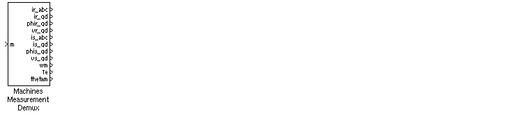
The Simulink output of the block is a vector containing 21 variables. They are, in order (refer to Description section above, all currents flowing into machine).

1-3: rotor currents i'_ra, i'_rb and i'_rc

4-9: i'_qr, i'_dr, '_qr, '_dr, v'_qr and v'_dr

10-12: stator currents i_sa, i_sb and i_sc

13-18: i_qs, i_ds, _qs, _ds, v_qs and v_ds

19-21: _m, T_e and _m

These variables can be demultiplexed by using the special Machines Measurement Demux block provided in the Machines library.

Limitations

The Asynchronous Machine block does not include a representation of the effects of stator and rotor iron saturation.

Example

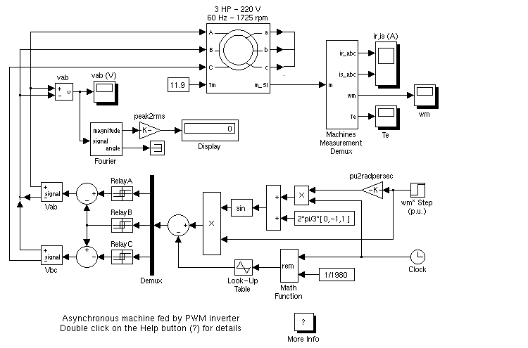
This example illustrates the use of the Asynchronous Machine block in motoring mode. It consists of an asynchronous machine in an open-loop speed control system. The machine's rotor is short-circuited and the stator is fed by a PWM inverter, which is built with Simulink blocks and interfaced to the Asynchronous Machine block through the Controlled Voltage Source block. The inverter uses sinusoidal pulse-width modulation, which is described in [2]. The base frequency of the sinusoidal reference wave is set at 60 Hz and the triangular carrier wave's frequency is set at 1980 Hz. This corresponds to a frequency modulation factor m_f of 33 (60 Hz x 33 = 1980). It is recommended in [2] that m_f be an odd multiple of three and that the value be as high as possible. The 3 HP machine is connected to a constant load of nominal value (11.9 N.m). It is started and reaches the setpoint speed of 1.0 p.u. at t=0.9 second. The parameters of the machine are those found in the SI Units dialog box above, except for the stator leakage inductance, which is set to twice its normal value. This is done to simulate a smoothing inductor placed between the inverter and the machine. Also, the stationary reference frame was used to obtain the results shown below.

Open the Simulink diagram by typing psbpwm or by choosing Asynchronous Machine from the Demos group in the powerlib library. Set the simulation parameters as follows:

Integrator type: Stiff, ode15s

Stop time: 1.0 s

Integration options: Use default options, except for Relative tolerance, which must be set to 1e-9. This relatively small tolerance is required because of the high switching rate of the inverter.

Run the simulation by choosing Start from the Simulation menu. Once the simulation is completed, observe the machine's speed and torque.

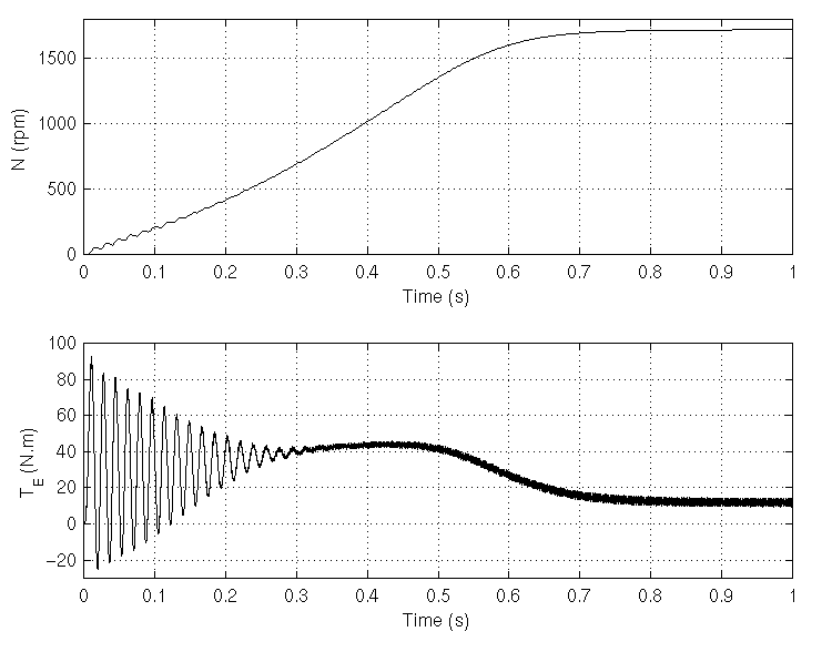
The top graph shows the machine's speed going from 0 to 1725 rpm (1.0 p.u.). The bottom graph shows the electromagnetic torque developed by the machine. Since the stator is fed by a PWM inverter, a noisy torque is observed.

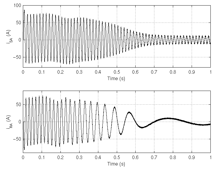
However, this noise is not visible in the speed since it is filtered out by the machine's inertia, but it can also be seen in the stator and rotor currents, which are observed next.

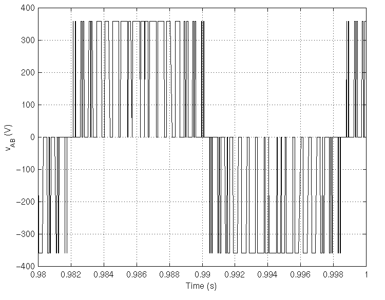
Finally, look at the output of the PWM inverter. Since nothing of interest can be seen at the simulation time scale, the graph concentrates on the last moments of the simulation.

References

[1] Krause P.C., O. Wasynczuk, S.D. Sudhoff, Analysis of Electric Machinery, IEEE Press, 1995.

[2] Mohan N., T.M. Undeland, W.P. Robbins, Power Electronics: Converters, Applications, and Design, John Wiley & Sons, Inc., 1995, section 8.4.1.

AC Voltage Source Breaker