vplot (Mu Analysis and Synthesis Toolbox)

Plot multiple VARYING matrices on the same graph

Syntax

vplot('plot_type',vmat1,vmat2,...) 
vplot('plot_type',vmat1,'linetype1',...) 
vplot('bode_l',top_axis_limits,bottom_axis_limits,vmat1,vmat2,...)

Description
The vplot command calls the standard MATLAB plot command for plotting. The optional plot_type argument specifies the type of graph, and selects between the various logarithmic or linear graph types. The plot_type specification choices are

iv,d
matrix (decimal) vs. independent variable

iv,m
magnitude vs. independent variable

iv,lm
log(magnitude) vs. independent variable

iv,p
phase vs. independent variable

liv,d
matrix vs. log(independent variable)

liv,m
magnitude vs. log(independent variable)

liv,lm
log(magnitude) vs. log(independent variable)

liv,p
phase vs. log(independent variable)

ri
real vs. imaginary (parametrized by independent variable)

nyq
real vs. imaginary (parametrized by independent variable)

nic
Nichols chart

bode
Bode magnitude and phase plots

bode_g
Bode magnitude and phase plots with grids

bode_l
Bode magnitude and phase plots with axis limits

bode_gl
Bode magnitude and phase plots with grids and axis limits

`iv,d`	matrix (decimal) vs. independent variable
`iv,m`	magnitude vs. independent variable
`iv,lm`	log(magnitude) vs. independent variable
`iv,p`	phase vs. independent variable
`liv,d`	matrix vs. log(independent variable)
`liv,m`	magnitude vs. log(independent variable)
`liv,lm`	log(magnitude) vs. log(independent variable)
`liv,p`	phase vs. log(independent variable)
`ri`	real vs. imaginary (parametrized by independent variable)
`nyq`	real vs. imaginary (parametrized by independent variable)
`nic`	Nichols chart
`bode`	Bode magnitude and phase plots
`bode_g`	Bode magnitude and phase plots with grids
`bode_l`	Bode magnitude and phase plots with axis limits
`bode_gl`	Bode magnitude and phase plots with grids and axis limits

If no plot_type specification is given the default is 'iv,d'.

The bode_l and bode_gl plot_type specifications require that the second and third arguments are the desired axis limits for the top and bottom plots. These are simply the 1x 4 vectors to be used as arguments for the axis command.

The remaining arguments of vplot take the same form as the MATLAB plot command. Line types (for example,'+', 'g-.', or '*r') can be optionally specified after any VARYING matrix argument.

There is a subtle distinction between CONSTANT and VARYING matrices with only one independent variable. A CONSTANT is treated as such across all independent variables, and consequently shows up as a line on any graph with the independent variable as an axis. A VARYING matrix with only one independent variable will always show up as a point. You may need to specify one of the more obvious point types in order to see it (e.g., '+', 'x', etc.).

Examples
Two SISO second-order systems are created, and their frequency responses are calculated for each over different frequency ranges.

a1 = [-1,1;-1,-0.5];
b1 = [0;2]; c1 = [1,0]; d1 = 0; 
sys1 = pck(a1,b1,c1,d1); 
minfo(sys1)
system:2 states1 outputs1 inputs
a2 = [-.1,1;-1,-0.05]; 
b2 = [1;1]; c2 = [-0.5,0]; d2 = 0.1; 
sys2 = pck(a2,b2,c2,d2); 
minfo(sys2)
system:2 states1 outputs1 inputs
omega = logspace(-2,2,100); 
sys1_g = frsp(sys1,omega); 
omega2 = [ [0.05:0.1:1.5] [1.6:.5:20] [0.9:0.01:1.1] ]; 
omega2 = sort(omega2); 
sys2_g2 = frsp(sys2,omega2);

A VARYING matrix with a single independent variable is also created. Note the distinction between this and the CONSTANT matrix in the subsequent plots.

rspot = vpck(sqrt(2)-sqrt(2)*i,2); 
minfo(rspot)
varying:1 pts1 rows1 cols

The following plot uses the 'liv,lm' plot_type specification. Note that the CONSTANT matrix is seen over all values of the independent variable. This is only true because it is displayed as a line type. If it were displayed as a point, then one would see points only on each of the side axes. The single valued VARYING matrix (rspot) is shown only at the appropriate independent variable value.

vplot('liv,lm',sys1_g,'b-.',[1+i;0.5-0.707*i],'g--',... 
rspot,'r*',sys2_g2);
xlabel('log independent variable') 
ylabel('log magnitude') 
title('plot_type specification: liv,lm')

You can customize vplot to select the type of axis uses for log magnitude and phase plots. The default is to plot the log magnitude on a base 10 scale and plot phase in radians. It is a simple modification to select a dB scale and phase in degrees. Documentation of the modification is provided in the M-file vplot. You can copy the command vplot to a private directory (for example, matlab/toolboxes/mu_cmds on UNIX systems) and make the appropriate modifications.

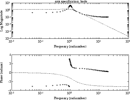
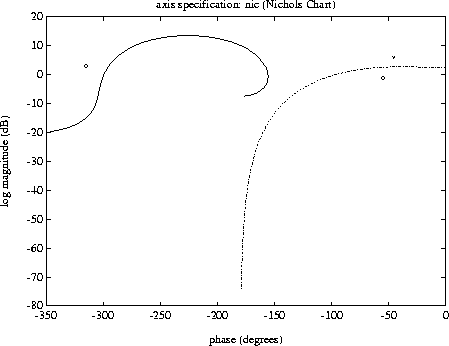
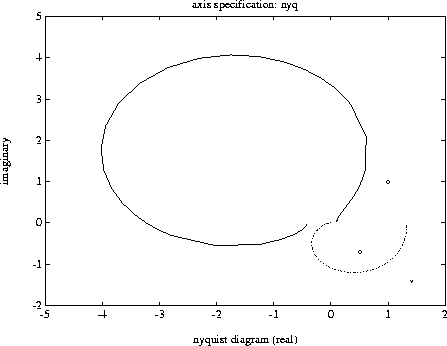
Several control design plot functions are also provided. These are bode, nic, and nyq, for Bode, Nichols, and Nyquist, respectively. The following three plots demonstrate each of these commands.

vplot('bode',sys1_g,'b',sys2_g2,'g+'); 
title('plot_type specification: bode')

The log magnitude and phase axes are labeled automatically. You can change these labels. Documentation for doing this is in the Help facility for vplot.

vplot('nic',sys1_g,'b-.',[1+i;0.5-0.707*i],'go',rspot,... 
rspot,'r*',sys2_g2);
title('plot_type specification: nic') 
xlabel('phase (degrees)') 
ylabel('log magnitude (dB)') 
title('plot_type specification: nic (Nichols Chart)')

The default axis scale selection for the Nichols plot is dB versus phase in degrees. This corresponds to the usual choice for this plot and can be different from the axis scale selection for bode, liv, lm, liv, p, etc. Again you can change this if required.

vplot('nyq',sys1_g,'b-.',[1+i;0.5-0.707*i],'go',rspot,... 
xlabel('nyquist diagram (real)') 
vplot('liv,lm',sys1_g,'b-.',[1+i;0.5-0.707*i],'g--',... 
rspot,'r*',sys2_g2);
ylabel('imaginary') 
title('plot_type specification: nyq')

See Also
plot

vpck, vunpck, var2con vpoly, vroots