| Model Predictive Control Toolbox | |
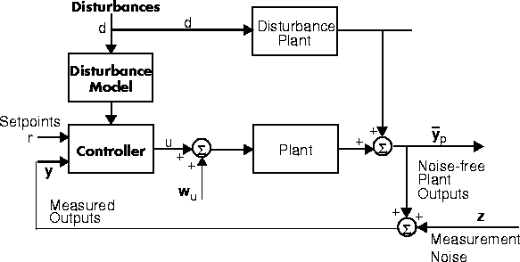
Combines a plant model and a controller model in MPC step format, yielding a closed-loop system model in the MPC mod format. This can be used for stability analysis and linear simulations of closed-loop performance.
Syntax
[clmod] =mpccl(plant,model,Kmpc) [clmod,cmod] =mpccl(plant,model,Kmpc,tfilter,...
dplant,dmodel)
plant
Is a model (in step format) representing the plant in the above diagram.
model
Is a model (in step format) that is to be used to design the MPC controller block shown in the diagram. It may be the same as plant (in which case there is no "model error" in the controller design), or it may be different.
Kmpc
Is a controller gain matrix, which was calculated by the function mpccon.
tfilter
Is a (optional) matrix of time constants for the noise filter and the unmeasured disturbances entering at the plant output. If omitted or set to an empty matrix, the default is no noise filtering and steplike unmeasured disturbances. See the documentation for the function mpcsim for more details on the design and proper format of tfilter.
dplant
Is a (optional) model (in step format) representing all the disturbances (measured and unmeasured) that affect plant in the above diagram. If omitted or set to an empty matrix, the default is that there are no disturbances.
dmodel
Is a (optional) model (in step format) representing the measured disturbances. If omitted or set to an empty matrix, the default is that there are no measured disturbances. See the documentation for the function mpcsim for more details on how disturbances are handled when using step-response models.
mpccl
Calculates a model of the closed-loop system, clmod. It is in the mod format and can be used, for example, with analysis functions such as smpcgain and smpcpole, and with simulation routines such as mod2step and dlsimm. mpccl also calculates (as an option) a model of the controller element, cmod.
clmod, has the following state-space representation:
 clxcl(k) +
  clucl(k)
ycl(k) = Cclxcl(k) + Dclucl(k)
cl, cl, Ccl, and Dcl are matrices of appropriate size. The expert user may want to know the significance of the state variables in xcl. They are (in the following order):
clucl(k)
ycl(k) = Cclxcl(k) + Dclucl(k)
cl, cl, Ccl, and Dcl are matrices of appropriate size. The expert user may want to know the significance of the state variables in xcl. They are (in the following order):
plant),
 d signal to yield a d signal. If there are no disturbances, these states are omitted.
wu signal to yield a wu signal.
u signal produced by the standard MPC formulation to yield a u signal that can be used as input to the plant and as a closed-loop output.
d signal to yield a d signal. If there are no disturbances, these states are omitted.
wu signal to yield a wu signal.
u signal produced by the standard MPC formulation to yield a u signal that can be used as input to the plant and as a closed-loop output.
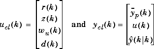
 is the estimate of the noise-free plant output at sampling period k based on information available at period k. This estimate is generated by the controller element.
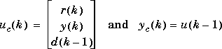
The state-space form of the controller model,
is the estimate of the noise-free plant output at sampling period k based on information available at period k. This estimate is generated by the controller element.
The state-space form of the controller model, cmod, can be written as:
cxc(k) + cuc(k)
yc(k) = Ccxc(k) + Dcuc(k)
Example
Consider the linear system:
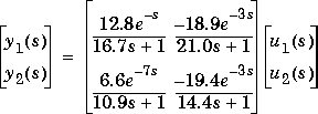
poly2tfd and tfd2step.
g11=poly2tfd(12.8,[16.7 1],0,1);
g21=poly2tfd(6.6,[10.9 1],0,7);
g12=poly2tfd(-18.9,[21.0 1],0,3);
g22=poly2tfd(-19.4,[14.4 1],0,3);
delt=3; ny=2; tfinal = 60;
model=tfd2step(tfinal,delt,ny,g11,g21,g12,g22);
plant=model; % No plant/model mismatch
Now we design the controller. Since there is delay, we use
M < P: We specify the defaults for the other tuning parameters, uwt and ywt, then calculate the controller gain:
P=6; % Prediction horizon.
M=2; % Number of moves (input horizon).
ywt=[ ]; % Output weights (default - unity
% on all outputs). uwt=[ ]; % Man. Var weights (default - zero
% on all man. vars).
Kmpc=mpccon(model,ywt,uwt,M,P);
Now we can calculate the model of the closed-loop system:
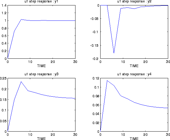
clmod=mpccl(plant,model,Kmpc);You can use the closed-loop model to calculate and plot the step response with respect to all the inputs. The appropriate commands are:
tend=30;
clstep=mod2step(clmod, tend);
plotstep(clstep)
Since the closed-loop system has m = 6 inputs and p = 6 outputs, only one of the plots is reproduced here. It shows the response of the first 4 closed-loop outputs to a unit step in the first closed-loop input, which is the setpoint for y1:
Restriction
model and plant must have been created using the same sampling period.
See Also
cmpc, mod2step, step format, mpccon, mpcsim, smpcgain, smpcpole
| mpcaugss | mpccon | |