Fixed-Point Blockset

Simulation 3: Automatic Scaling

Using the automatic scaling procedure, you can easily maximize the precision of the output data type while spanning the full simulation range. For a complex model, the absence of such a procedure can make achieving this goal tedious and time consuming.

Automatic scaling is performed for the Controller block. This block is a subsystem representing software running on the target, and requires optimization. Automatic scaling consists of these steps:

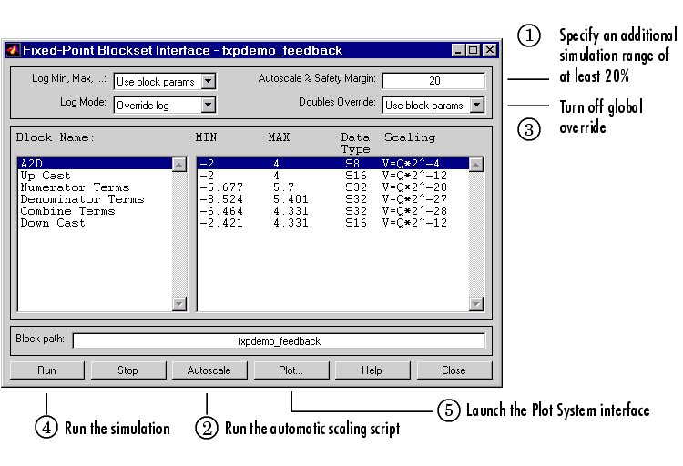
1. Configure Autoscale % Safety Margin to 20. This sets scaling so that the largest simulation value seen is at least 20% smaller than the maximum value allowed.

The Autoscale % Safety Margin parameter value multiplies the "raw" simulation values by a factor of 1.2. Configuring this parameter to a value greater than 1 guarantees the simulation covers the largest possible range, although it does not necessarily mean the resolution improves. Since there is always some uncertainty when representing a real-world value with a fixed-point number with only a few simulations, using this parameter is recommended.

2. Run the autofixexp M-file script by selecting the Autoscale button. This script automatically changes the scaling on all fixed-point blocks that do not have their scaling locked, and that have their output data type specified as a generalized fixed-point number. It uses the minimum and maximum data logged from the previous simulation. The scaling changes such that the precision is maximized while the full range of simulation values are spanned for each block.
3. Turn off the global override with doubles by configuring Doubles Override to Use block params.
4. Run the simulation by selecting the Run button. The automatic scaling results generated by step 2 are captured from the MATLAB workspace and applied to the simulation.
5. Launch the Plot System interface and plot the plant output signal.

The procedure and results for this simulation are shown below.

Each block is scaled based on its own maximum and minimum values obtained from the previous simulation using double-precision numbers. As shown above, the interface displays the new scaling for each block that had its scaling changed. This scaling is based on the raw simulation values multiplied by 1.2. Note that no saturations or overflows are reported.

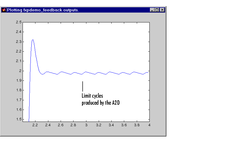
A close-up of the plant output signal is shown below. Note that a steady-state has been achieved, but a small limit cycle is present in the steady state due to poor A/D design.

As shown below, the scaling of the A2D did not change because it was locked.

Simulation 2: Global Override

Simulation 4: Individual Override