Fixed-Point Blockset

Example: Constant Scaling for Best Precision

The Fixed-Point Blockset provides you with block-specific modes for scaling constant vectors and constant matrices. These scaling modes are based on radix point-only scaling and are described below:

• Constant Vector Scaling

Using this mode, you can scale a constant vector such that its precision is maximized element-by-element, or a common radix point is found based on the best precision for the largest value of the vector.

• Constant Matrix Scaling

Using this mode, you can scale a constant matrix such that its precision is maximized element-by-element, or a common radix point is found based on the best precision for the largest value of each row, each column, or the whole matrix.

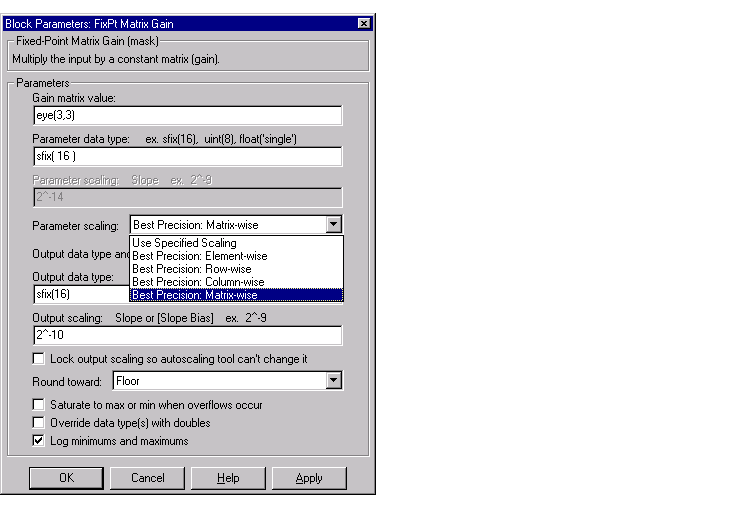
Constant matrix and constant vector scaling are available only for generalized fixed-point data types. All other fixed-point data types use their default scaling. The available constant matrix scaling modes are shown below for the FixPt Matrix Gain block.

To understand how you might use these scaling modes, consider a 5 by 4 matrix of doubles, M, defined as

  3.3333e-005  3.3333e-006  3.3333e-007  3.3333e-008
  3.3333e-004  3.3333e-005  3.3333e-006  3.3333e-007
  3.3333e-003  3.3333e-004  3.3333e-005  3.3333e-006
  3.3333e-002  3.3333e-003  3.3333e-004  3.3333e-005
  3.3333e-001  3.3333e-002  3.3333e-003  3.3333e-004

Now suppose M is input into the FixPt Matrix Gain block, and you want to scale it using one of the constant matrix scaling modes. The results of using these modes are described below:

• Use Specified Scaling

Suppose the matrix elements are converted to a signed, 10-bit generalized fixed-point data type with radix point-only scaling of 2^-7 (that is, the radix point is located seven places to the left of the rightmost bit). With this data format, M becomes

0            0           0            0
0            0           0            0
0            0           0            0
3.1250e-002  0           0            0
3.3594e-001  3.1250e-002 0            0

Note that many of the matrix elements are zero, and for the nonzero entries, the scaled values differ from the original values. This is because a double is converted to a binary word of fixed size and limited precision for each element. The larger and more precise the conversion data type, the more closely the scaled values match the original values.

• Best Precision: Element-wise

If M is scaled such that the precision is maximized for each matrix element, you obtain

3.3379e-005  3.3304e-006  3.3341e-007  3.3295e-008
3.3379e-004  3.3379e-005  3.3304e-006  3.3341e-007
3.3340e-003  3.3379e-004  3.3379e-005  3.3304e-006
3.3325e-002  3.3340e-003  3.3379e-004  3.3379e-005
3.3301e-001  3.3325e-002  3.3340e-003  3.3379e-004

• Best Precision: Row-wise

If M is scaled based on the largest value for each row, you obtain

3.3379e-005  3.3379e-006  3.5763e-007 0
3.3379e-004  3.3379e-005  2.8610e-006 0
3.3340e-003  3.3569e-004  3.0518e-005 0
3.3325e-002  3.2959e-003  3.6621e-004 0
3.3301e-001  3.3203e-002  2.9297e-003 0

• Best Precision: Column-wise

If M is scaled based on the largest value for each column, you obtain

0            0            0            0
0            0            0            0
2.9297e-003  3.6621e-004  3.0518e-005  2.8610e-006
3.3203e-002  3.2959e-003  3.3569e-004  3.3379e-005
3.3301e-001  3.3325e-002  3.3340e-003  3.3379e-004

• Best Precision: Matrix-wise

If M is scaled based on its largest matrix value, you obtain

0            0            0            0
0            0            0            0
2.9297e-003  0            0            0
3.3203e-002  2.9297e-003  0            0
3.3301e-001  3.3203e-002  2.9297e-003  0

The disadvantage of scaling the matrix column-wise, row-wise, or matrix-wise is reduced precision resulting from the use of a common radix point. The advantage of using a common radix point is reduced code size and possibly increased processor speed.

Example: Fixed-Point Scaling

Floating-Point Numbers