
| Financial Toolbox |   |
Plotting Sensitivities of an Option
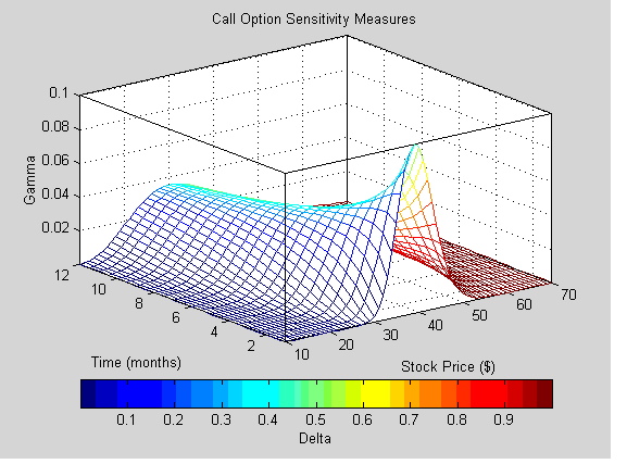
This example creates a three-dimensional plot showing how gamma changes relative to price for a Black-Scholes option. Recall that gamma is the second derivative of the option price relative to the underlying security price. The plot shows a three-dimensional surface whose z-value is the gamma of an option as price (x-axis) and time (y-axis) vary. It adds yet a fourth dimension by showing option delta (the first derivative of option price to security price) as the color of the surface. This example M-file is ftgex2.m.
Range = 10:70;
Span = length(Range);
j = 1:0.5:12;
Newj = j(ones(Span,1),:)'/12;
For each time period create a vector of prices from 10 to 70 and create a matrix of all ones.
JSpan = ones(length(j),1);
NewRange = Range(JSpan,:);
Pad = ones(size(Newj));
Call the toolbox gamma and delta sensitivity functions. Exercise price is $40, risk-free interest rate is 10%, and volatility is 0.35 for all prices and periods. Gamma is the z-axis, delta is the color.
ZVal = blsgamma(NewRange, 40*Pad, 0.1*Pad, Newj, 0.35*Pad);
Color = blsdelta(NewRange, 40*Pad, 0.1*Pad, Newj, 0.35*Pad);
Draw the surface as a mesh, add axis labels and a title. The axes range from 10 to 70, 1 to 12, and -
 to
to  .
.
mesh(Range, j, ZVal, Color);
xlabel('Stock Price ($)');
ylabel('Time (months)');
zlabel('Gamma');
title('Call Option Sensitivity Measures');
axis([10 70  1 12  -inf inf]);
Finally add a box around the whole plot, annotate the colors with a bar, and label the colorbar.
set(gca, 'box', 'on');
colorbar('horiz');
a = findobj(gcf, 'type', 'axes');
set(get(a(2), 'xlabel'), 'string', 'Delta');

 | Producing Graphics with the Toolbox | Plotting Sensitivities of a Portfolio of Options |  |