
| Financial Toolbox |   |
Sensitivity of Bond Prices to Parallel Shifts in the Yield Curve
Often bond portfolio managers want to consider more than just the sensitivity of a portfolio's price to a small shift in the yield curve, particularly if the investment horizon is long. This example shows how MATLAB can visualize the price behavior of a portfolio of bonds over a wide range of yield curve scenarios, and as time progresses toward maturity.
ftspex3.m.
Step 1.
Specify values for the settlement date, maturity date, face value, coupon rate, and coupon payment periodicity of a four-bond portfolio. For simplicity, accept default values for the end-of-month payment rule (rule in effect) and day-count basis (actual/actual). Also, synchronize the coupon payment structure to the maturity date (no odd first or last coupon dates). Any inputs for which defaults are accepted are set to empty matrices ([]) as placeholders where appropriate.
Settle     = '15-Jan-1995';
Maturity   = datenum(['03-Apr-2020'; '14-May-2025'; ...
                      '09-Jun-2019'; '25-Feb-2019']);
Face       = [1000; 1000; 1000; 1000];
CouponRate = [0; 0.05; 0; 0.055];
Periods    = [0; 2; 0; 2];
Also, specify the points on the yield curve for each bond.
Yields = [0.078; 0.09; 0.075; 0.085];
Step 2. Use Financial Toolbox functions to calculate the true bond prices as the sum of the quoted price plus accrued interest.
[CleanPrice, AccruedInterest] = bndprice(Yields,...
CouponRate,Settle, Maturity, Periods,...
[], [], [], [], [], [], Face);

Prices  =  CleanPrice + AccruedInterest;
Step 3. Assume the value of each bond is $25,000, and determine the quantity of each bond such that the portfolio value is $100,000.
BondAmounts = 25000 ./ Prices;
Step 4.
Compute the portfolio price for a rolling series of settlement dates over a range of yields. The evaluation dates occur annually on January 15, beginning on 15-Jan-1995 (settlement) and extending out to 15-Jan-2018. Thus, this step evaluates portfolio price on a grid of time of progression (dT) and interest rates (dY).
dy = -0.05:0.005:0.05;               % Yield changes

D  = datevec(Settle);                % Get date components
dt = datenum(D(1):2018, D(2), D(3)); % Get evaluation dates

[dT, dY]  =  meshgrid(dt, dy); % Create grid

NumTimes  =  length(dt);       % Number of time steps
NumYields =  length(dy);       % Number of yield changes
NumBonds  =  length(Maturity); % Number of bonds

% Preallocate vector
Prices = zeros(NumTimes*NumYields, NumBonds);
Now that the grid and price vectors have been created, compute the price of each bond in the portfolio on the grid one bond at a time.
for i = 1:NumBonds

   [CleanPrice, AccruedInterest] = bndprice(Yields(i)+...
   dY(:), CouponRate(i), dT(:), Maturity(i), Periods(i),...
   [], [], [], [], [], [], Face(i));

   Prices(:,i) = CleanPrice + AccruedInterest;

end
Scale the bond prices by the quantity of bonds.
Prices = Prices * BondAmounts;Reshape the bond values to conform to the underlying evaluation grid.
Prices = reshape(Prices, NumYields, NumTimes);
Step 5.
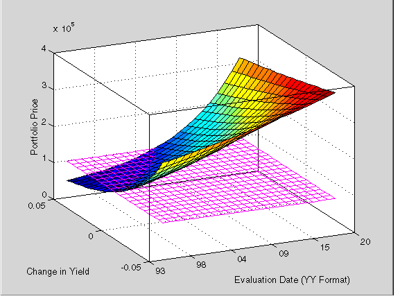
Plot the price of the portfolio as a function of settlement date and a range of yields, and as a function of the change in yield (dY). This plot illustrates the interest rate sensitivity of the portfolio as time progresses (dT), under a range of interest rate scenarios. With the following graphics commands, you can visualize the three-dimensional surface relative to the current portfolio value (i.e., $100,000).
figure                   % Open a new figure window
surf(dt, dy, Prices)     % Draw the surface
Add the base portfolio value to the existing surface plot.
hold on                  % Add the current value for reference
basemesh = mesh(dt, dy, 100000*ones(NumYields, NumTimes));
Make it transparent, plot it so the price surface shows through, and draw a box around the plot.
set(basemesh, 'facecolor', 'none');
set(basemesh, 'edgecolor', 'm');
set(gca, 'box', 'on');
Plot the x-axis using two-digit year (YY format) labels for ticks.
dateaxis('x', 11);
Add axis labels and set the three-dimensional viewpoint. MATLAB produces the figure.
xlabel('Evaluation Date (YY Format)');
ylabel('Change in Yield');
zlabel('Portfolio Price');
hold off
view(-25,25);

MATLAB's three-dimensional graphics allow you to visualize the interest rate risk experienced by a bond portfolio over time. This example assumed parallel shifts in the term structure, but it might similarly have allowed other components to vary, such as the level and slope.
 | Constructing a Bond Portfolio to Hedge Against Duration and Convexity | Constructing Greek-Neutral Portfolios of European Stock Options |  |