

| Excel Link |   |
This section shows how Microsoft Excel, Excel Link, and MATLAB work together to solve real-world problems.
These examples ship with Excel Link in the fileEXLISAMP.XLS, which is installed in the subdirectory EXLINK under your MATLAB directory (for example C:\MATLAB\EXLINK). Start Excel, Excel Link, and MATLAB. Open and try executing the examples.
| Note: Examples 1 and 2 use only basic MATLAB functions. Examples 3, 4, and 5 use functions in the optional MATLAB Financial Toolbox. |
Example 1: Regression and Curve Fitting
Regression techniques and curve fitting attempt to find functions that describe the relationship among variables. In effect, they attempt to build mathematical models of a data set. MATLAB provides many powerful yet easy-to-use matrix operators and functions to simplify the task.
Worksheet Version
To try the worksheet-only version of this example, click the Sheet1 tab on EXLISAMP.XLS.
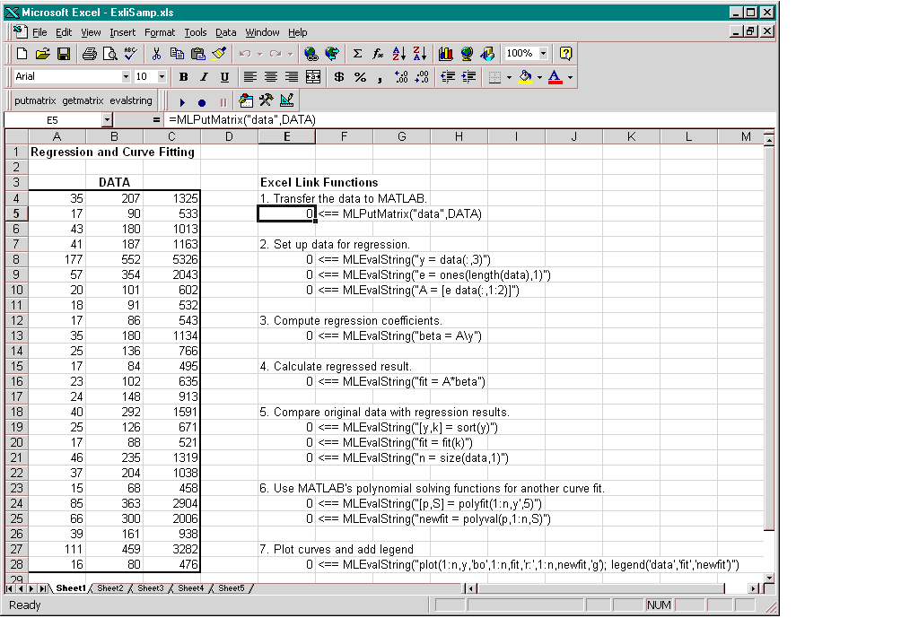
The worksheet contains one named range: A4:C28 is named DATA and contains the sample data set.
E5 the active cell. Press F2, then Enter to execute the Excel Link function that copies the sample data set to MATLAB. The data set contains 25 observations of three variables. There is a strong linear dependence among the observations; in fact, they are close to being scalar multiples of each other.
E8 and press F2, then Enter. Repeat with cells E9 and E10. These Excel Link functions tell MATLAB to regress the third column of data on the other two columns. They create a single vector y containing the third-column data, and a new three-column matrix A consisting of a column of ones followed by the rest of the data.
E13. This function computes the regression coefficients by using the MATLAB backslash operation to solve the (overdetermined) system of linear equations, A*beta = y.
E16. MATLAB matrix-vector multiplication produces the regressed result (fit).
E19, E20, and E21. These functions compare the original data with fit; sort the data in increasing order and apply the same permutation to fit; and create a scalar for the number of observations.
E24 and E25. Often it is useful to fit a polynomial equation to data. To do so, you would ordinarily have to set up a system of simultaneous linear equations and solve for the coefficients. The MATLAB polyfit function automates this procedure, in this case for a fifth-degree polynomial. The polyval function then evaluates the resulting polynomial at each data point to check the goodness of fit (newfit).
E28. The MATLAB plot function graphs the original data (blue circles), the regressed result fit (dashed red line), and the polynomial result (solid green line); and adds a legend
.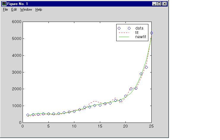
fit curve (dashed line) shows a close, but not an exact, fit. The fifth-degree polynomial curve, newfit, represents a more accurate mathematical model for the data.
When you have finished with this version of the example, close the figure window.
Macro Version
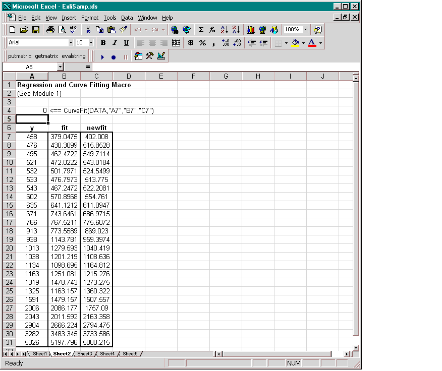
To try the macro-and-worksheet version of this example, click the Sheet2 tab on EXLISAMP.XLS.
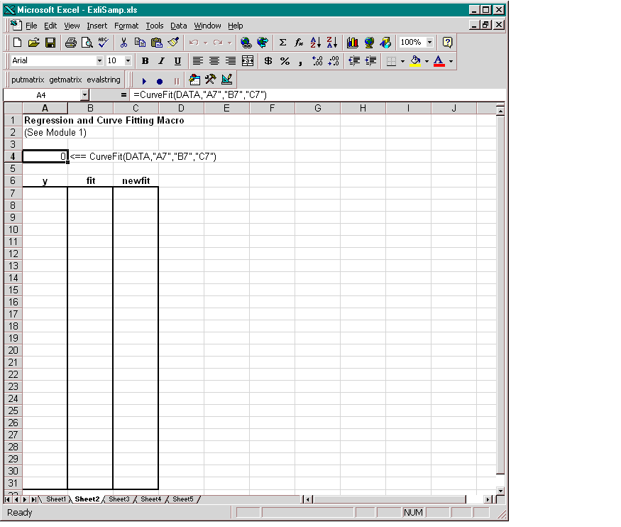
Make cell A4 the active cell, but do not execute it yet.
A4 calls the macro CurveFit, which you can examine from the Visual Basic environment.
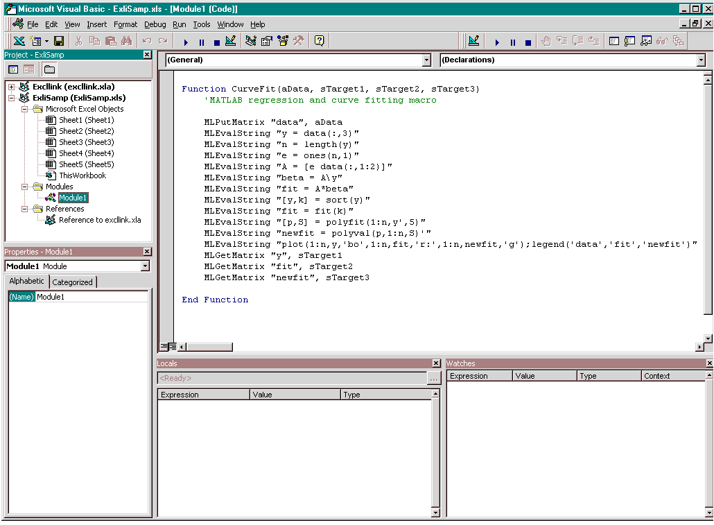
While this module is open, pull down the Tools menu and select References. In the References window, make sure there is a check in the box for EXCLLINK.XLA. If not, check the box and click OK. You may have to use Browse... to find the EXCLLINK.XLA file.
A4 of Sheet2, press F2, then Enter to execute the CurveFit macro. The macro executes the same functions as in Step 1 through Step 7 of the worksheet version (in a slightly different order), including plotting the graph. Plus, it copies the original data y (sorted), the corresponding regressed data fit, and the polynomial data newfit, to the worksheet. (The last three MLGetMatrix functions in the CurveFit macro copy data to the Excel worksheet.)
When you have finished with the example, close the figure window.
 | Using Excel Link | Example 2: Interpolating Data |  |