Design Case Studies

Hard-Disk Read/Write Head Controller

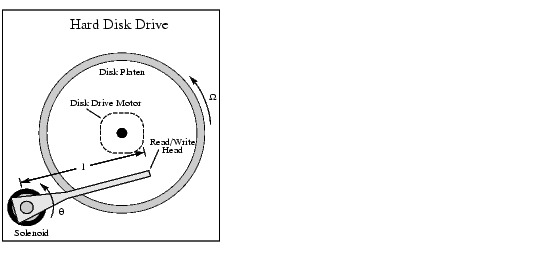
This case study demonstrates the ability to perform classical digital control design by going through the design of a computer hard-disk read/write head position controller.

Using Newton's law, a simple model for the read/write head is the differential equation

where is the inertia of the head assembly, is the viscous damping coefficient of the bearings, is the return spring constant, is the motor torque constant, is the angular position of the head, and is the input current.

Taking the Laplace transform, the transfer function from to is

Using the values kg , Nm/(rad/sec), Nm/rad, and Nm/rad, form the transfer function description of this system. At the MATLAB prompt, type

J = .01; C = 0.004; K = 10; Ki = .05;
num = Ki;
den = [J C K];
H = tf(num,den)

MATLAB responds with

Transfer function:
         0.05
-----------------------
0.01 s^2 + 0.004 s + 10

The task here is to design a digital controller that provides accurate positioning of the read/write head. The design is performed in the digital domain. First, discretize the continuous plant. Because our plant will be equipped with a digital-to-analog converter (with a zero-order hold) connected to its input, use c2d with the 'zoh' discretization method. Type

Ts = 0.005;     % sampling period = 0.005 second
Hd = c2d(H,Ts,'zoh')
Transfer function:
6.233e-05 z + 6.229e-05
-----------------------
 z^2 - 1.973 z + 0.998
 
Sampling time: 0.005

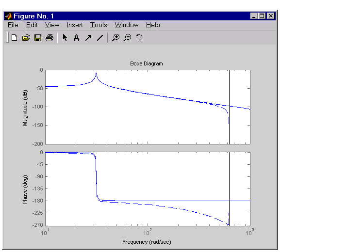
You can compare the Bode plots of the continuous and discretized models with

bode(H,'-',Hd,'--')

To analyze the discrete system, plot its step response, type

step(Hd)

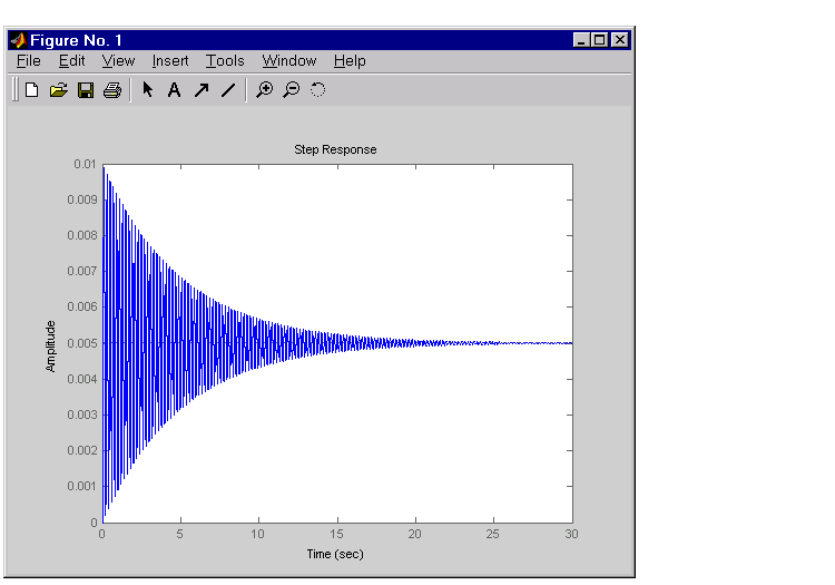
The system oscillates quite a bit. This is probably due to very light damping. You can check this by computing the open-loop poles. Type

% Open-loop poles of discrete model
damp(Hd) 
    Eigenvalue         Magnitude    Equiv. Damping    Equiv. Freq.
                                                                               
9.87e-01 + 1.57e-01i     9.99e-01         6.32e-03             3.16e+01        
9.87e-01 - 1.57e-01i     9.99e-01         6.32e-03             3.16e+01        

The poles have very light equivalent damping and are near the unit circle. You need to design a compensator that increases the damping of these poles.

The simplest compensator is just a gain, so try the root locus technique to select an appropriate feedback gain.

rlocus(Hd)

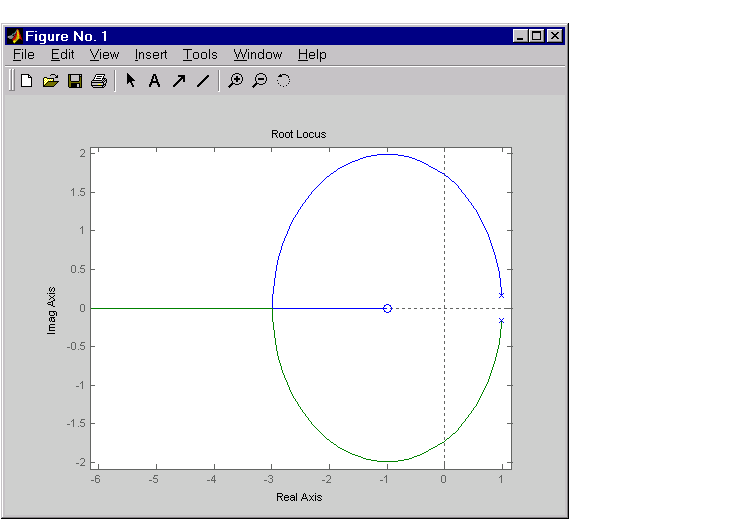
As shown in the root locus, the poles quickly leave the unit circle and go unstable. You need to introduce some lead or a compensator with some zeros. Try the compensator

with and .

The corresponding open-loop model

is obtained by the series connection

D = zpk(0.85,0,1,Ts)
oloop = Hd * D

Now see how this compensator modifies the open-loop frequency response.

bode(Hd,'--',oloop,'-')

The plant response is the dashed line and the open-loop response with the compensator is the solid line.

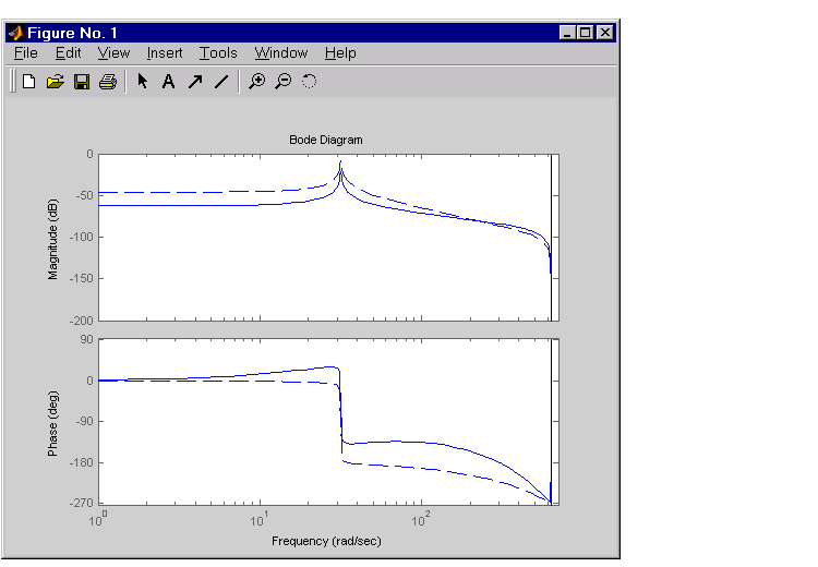
The plot above shows that the compensator has shifted up the phase plot (added lead) in the frequency range rad/sec.

Now try the root locus again with the plant and compensator as open loop.

rlocus(oloop)
zgrid

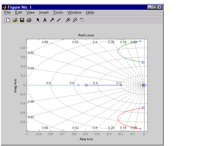
Open the Property Editor by right-clicking in the plot away from the curve. On the Limits page, set the x-axis limits from -1 to 1.01. This figure shows the result.

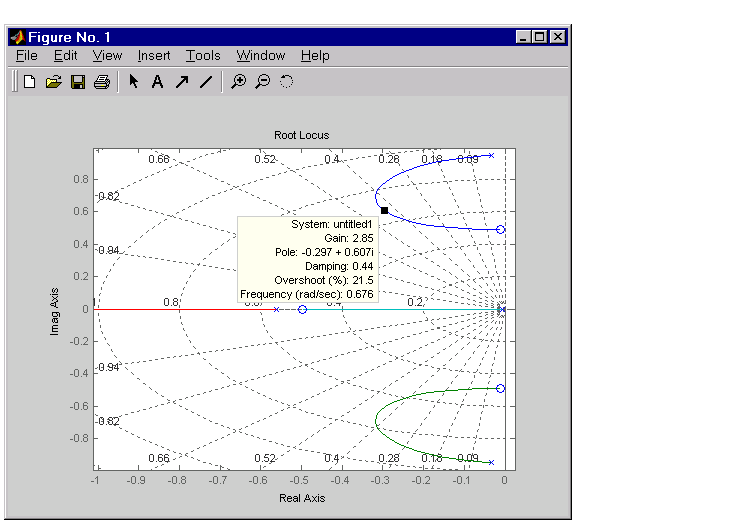
This time, the poles stay within the unit circle for some time (the lines drawn by zgrid show the damping ratios from to 1 in steps of 0.1). Use a data marker to find the point on the curve where the gain equals 4.111e+03. This figure shows the data marker at the correct location.

To analyze this design, form the closed-loop system and plot the closed-loop step response.

K = 4.11e+03;
cloop = feedback(oloop,K);
step(cloop)

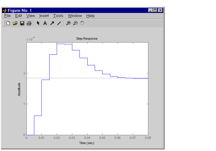
This response depends on your closed loop set point. The one shown here is relatively fast and settles in about 0.07 seconds. Therefore, this closed loop disk drive system has a seek time of about 0.07 seconds. This is slow by today's standards, but you also started with a very lightly damped system.

Now look at the robustness of your design. The most common classical robustness criteria are the gain and phase margins. Use the function margin to determine these margins. With output arguments, margin returns the gain and phase margins as well as the corresponding crossover frequencies. Without output argument, margin plots the Bode response and displays the margins graphically.

To compute the margins, first form the unity-feedback open loop by connecting the compensator , plant model, and feedback gain in series.

olk = K * oloop;

Next apply margin to this open-loop model. Type

[Gm,Pm,Wcg,Wcp] = margin(olk);
Margins = [Gm Wcg Pm Wcp]
Margins =

    3.7987  296.7978   43.2031  106.2462

To obtain the gain margin in dB, type

20*log10(Gm)
ans =
   11.5926

You can also display the margins graphically by typing

margin(olk)

The command produces the plot shown below.

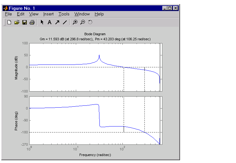
This design is robust and can tolerate a 11 dB gain increase or a 40 degree phase lag in the open-loop system without going unstable. By continuing this design process, you may be able to find a compensator that stabilizes the open-loop system and allows you to reduce the seek time.

Washout Filter Design

LQG Regulation: Rolling Mill Example