Graphics

Combining Stem Plots with Line Plots

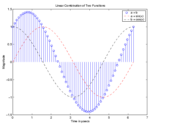
Sometimes it is useful to display more than one plot simultaneously with a stem plot to show how you arrived at a result. For example, create a linearly spaced vector with 60 elements and define two functions, a and b.

x = linspace(0,2*pi,60);
a = sin(x);
b = cos(x);

Create a stem plot showing the linear combination of the two functions.

stem_handles = stem(x,a+b);

Overlaying a and b as line plots helps visualize the functions. Before plotting the two curves, set hold to on so MATLAB does not clear the stem plot.

hold on
plot_handles = plot(x,a,'--r',x,b,'--g');
hold off

Use legend to annotate the graph. The stem and plot handles passed to legend identify which lines to label. Stem plots are composed of two lines; one draws the markers and the other draws the vertical stems. To create the legend, use the first handle returned by stem, which identifies the marker line.

legend_handles = [stem_handles(1);plot_handles];
legend(legend_handles,'a + b','a = sin(x)','b = cos(x)')

Labeling the axes and creating a title finishes the graph.

xlabel('Time in \musecs')
ylabel('Magnitude')
title('Linear Combination of Two Functions')

 

Two-Dimensional Stem Plots

Three-Dimensional Stem Plots