Wavelet analysis example
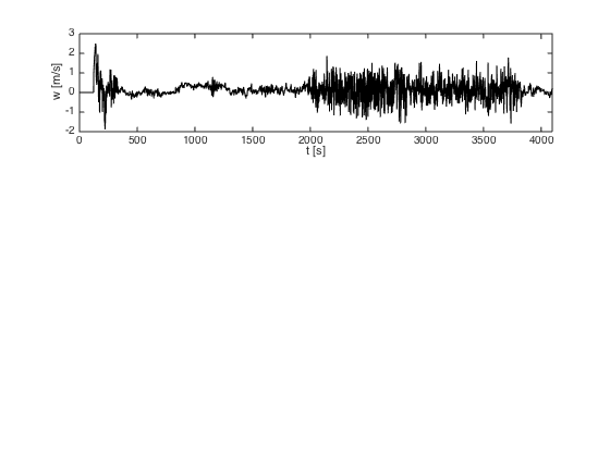
Haar wavelet analysis of a nonstationary dataset of aircraft-measured vertical velocity measured each second while the plane moved up and down through the lower layers of the atmosphere.
Contents
Load, subset and plot data
  clear all
  load w_VOCALSRF03;
  whos

  N= 4096;
  w = w(1:N); % Subset to first 4096 samples for simplicity

  figure(1)
  clf
  subplot(3,1,1)
  plot(w,'k')  % Note that data is quite nonstationary
  xlim([0 N])
  xlabel('t [s]')
  ylabel('w [m/s]')
  Name          Size             Bytes  Class     Attributes

  w         30241x1             241928  double
Plot level-1 Haar transform of s
  [cA1,cD1] = dwt(w,'db1');  % Single-level Haar (db1) wavelet transform
  A1 = upcoef('a',cA1,'db1',1,N); % Average time series
  D1 = upcoef('d',cD1,'db1',1,N); % Detail time series

  subplot(3,1,2)
  plot(1:N/2,cA1,'b',(N/2+1):N,cD1,'r')
  xlim([0 N])
  legend('a^1','d^1')
  ylabel('1-level Haar DWT')

Plot partitioning of signal into average and detail components.
  subplot(3,1,3)
  plot(1:N,A1,'b',1:N,D1,'r')
  xlim([0 N])
  legend('A^1','D^1')
  ylabel('Partitioning of signal')

3-level Haar transform
  figure(2)
  clf

  [C,L] = wavedec(w,3,'db1');
  A3 = wrcoef('a',C,L,'db1',3);
  D1 = wrcoef('d',C,L,'db1',1);
  D2 = wrcoef('d',C,L,'db1',2);
  D3 = wrcoef('d',C,L,'db1',3) ;

  % Plot level-3 Haar transform

  subplot(3,1,1)
  plot(1:N/8,C(1:N/8),'b',(N/8+1):(N/4),C((N/8+1):(N/4)),'c',...
       (N/4+1):(N/2),C((N/4+1):(N/2)),'m',...
       (N/2+1):N,C((N/2+1):N),'r')
  xlim([0 N])
  ylabel('3-level Haar DWT')
  legend('a^3','d^3','d^2','d^1')

  % Plot signal and the 3rd level averaged signal

  subplot(3,1,2)
  plot(1:N,w,'k',1:N,A3,'b')
  xlim([0 N])
  legend('signal','A^3')


  % Plot the three detail components of signal

  subplot(3,1,3)
  yoff = 2;
  plot(1:N,D1,'r',1:N,D2+yoff,'m',1:N,D3+2*yoff,'c')
  xlim([0 N])
  ylim([-yoff,3*yoff])
  legend('D1','D2','D3')

Wavelet power averaged over 64-s windows
Nw = 64;
nwins = N/Nw;
tw = Nw*((1:nwins) - 0.5);  % Time at window centers
A3pow = mean(reshape(A3.^2,Nw,nwins));
D3pow = mean(reshape(D3.^2,Nw,nwins));
D2pow = mean(reshape(D2.^2,Nw,nwins));
D1pow = mean(reshape(D1.^2,Nw,nwins));

figure(3)
clf
subplot(3,1,1)
plot(tw,D1pow,'r.',...
     tw,D1pow+D2pow,'m.',...
     tw,D1pow+D2pow+D3pow,'c.',...
     tw,D1pow+D2pow+D3pow+A3pow,'b.')
xlim([0 N])
xlabel('t [s]')
ylabel('var(w) [m^2s^{-2}]')
legend('D1','+D2','+D3','+A3')

CWT example
  scale = 2.^((1:40)/4);
  W = cwt(w,scale,'haar');
  figure(4)
  clf
  image(1:N,(1:40)/4,W,'CDataMapping','scaled')
  title('CWT of w - vertical axis is log2(scale)')
  xlabel('t [s]')
  ylabel('log2(scale)')
  axis xy
