Wavelet analysis example from Matlab wavelet toolbox

Make plots for wavelet example from Matlab toolbox using electrical consumption time series leleccum (sampling rate 1/minute; tabulated over 2.7 days)

Contents

Load data

  load leleccum;
  s = leleccum(1:4096);
  ls = length(s);

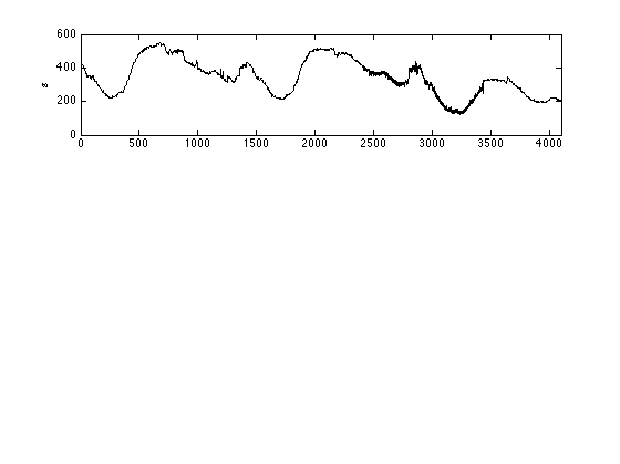
Plot signal

  figure(1)
  subplot(3,1,1)
  plot(s,'k')
  v = axis;
  v(1:2) = [0 ls];
  axis(v);
  ylabel('s')

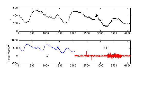
Plot level-1 Haar transform of s

  [cA1,cD1] = dwt(s,'db1');  % Single-level Haar (db1) wavelet transform
  A1 = upcoef('a',cA1,'db1',1,ls); % Average time series
  D1 = upcoef('d',cD1,'db1',1,ls); % Detail time series

  subplot(3,1,2)
  plot(1:ls/2,cA1,'b',(ls/2+1):ls,10*cD1,'r')
  v = axis;
  v(1:2) = [0 ls];
  axis(v);
  text(ls/4,0,'a^1')
  text(3*ls/4,500,'10d^1')
  ylabel('1-level Haar DWT')

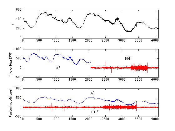
Plot partitioning of signal into average and detail components.

  subplot(3,1,3)
  plot(1:ls,A1,'b',1:ls,10*D1,'r')
  v = axis;
  v(1:2) = [0 ls];
  axis(v);
   text(ls/2,750,'A^1')
  text(ls/2,-250,'10D^1')
  ylabel('Partitioning of signal')

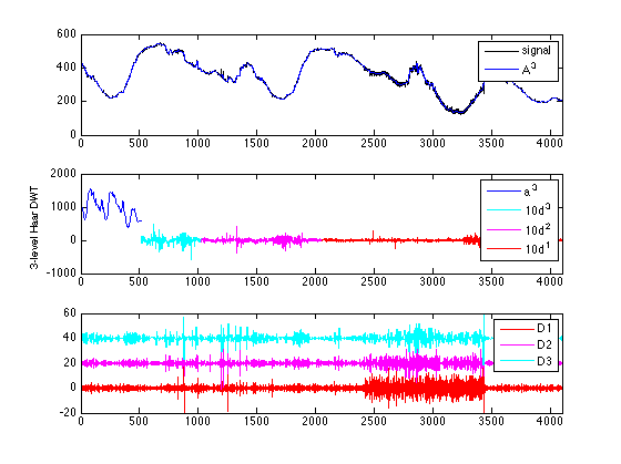
3-level Haar transform

  figure(2)
  [C,L] = wavedec(s,3,'db1');
  A3 = wrcoef('a',C,L,'db1',3);
  D1 = wrcoef('d',C,L,'db1',1);
  D2 = wrcoef('d',C,L,'db1',2);
  D3 = wrcoef('d',C,L,'db1',3) ;

  % Plot signal and the 3rd level averaged signal

  subplot(3,1,1)
  plot(1:ls,s,'k',1:ls,A3,'b')
  v = axis;
  v(1:2) = [0 ls];
  axis(v);
  legend('signal','A^3')

  % Plot level-3 Haar transform

  subplot(3,1,2)
  plot(1:ls/8,C(1:ls/8),'b',(ls/8+1):(ls/4),10*C((ls/8+1):(ls/4)),'c',...
       (ls/4+1):(ls/2),10*C((ls/4+1):(ls/2)),'m',...
       (ls/2+1):ls,10*C((ls/2+1):ls),'r')
  v = axis;
  v(1:2) = [0 ls];
  axis(v);
   ylabel('3-level Haar DWT')
  legend('a^3','10d^3','10d^2','10d^1')

  % Plot the three detail components of signal

  subplot(3,1,3)
  yoff = 20;
  plot(1:ls,D1,'r',1:ls,D2+yoff,'m',1:ls,D3+2*yoff,'c')
  v = axis;
  v(1:2) = [0 ls];
  axis(v);
;   axis([0,ls,-20,60])
  legend('D1','D2','D3')

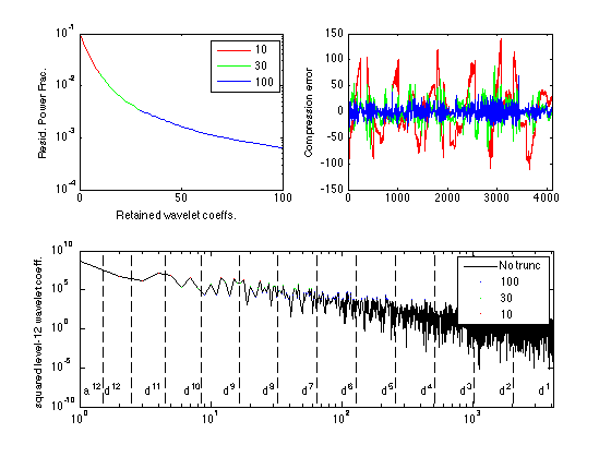
Signal compression

  p = log2(ls);
  s2 = leleccum(1:ls);

  % Calculate complete p-level Haar transform

  [C,L] = wavedec(s2,p,'db1');

  % Plot the largest nkeep wavelet coefficients, for various
  % choices nkeep

  figure(3)
  subplot(2,2,1)
  Csq = C.^2;
  [mCsqsort,Isort] = sort(-Csq);  % Tricky way to sort wavelet coeffs from
                                % largest to smallest in magnitude.
  cumpow = cumsum(mCsqsort)/sum(mCsqsort); % Cum frac of Wavelet power
  nkeep = [10 30 100];
  semilogy(1:nkeep(1),1-cumpow(1:nkeep(1)),'r',...
           nkeep(1):nkeep(2),1-cumpow(nkeep(1):nkeep(2)),'g',...
           nkeep(2):nkeep(3),1-cumpow(nkeep(2):nkeep(3)),'b');
  xlabel('Retained wavelet coeffs.')
  ylabel('Resid. Power Frac.')
  legend(int2str(nkeep(1)),int2str(nkeep(2)),int2str(nkeep(3)))

  % Reconstruct signal if other wavelet coeffs are zeroed out and
  % plot 'compression error' in the signal that this induces.

  subplot(2,2,2)
  col = 'rgb';  % Vector of plotting colors
  for ik = 1:length(nkeep)
    jsort = Isort(1:nkeep(ik));
    C2 = C - C;  % Zero wavelet coeffs of compressed signal
    C2(jsort) = C(jsort); % ...except for the nkeep(ik) largest.
    sc = waverec(C2,L,'db1'); % Reconstruction after compression
    plot(1:ls, sc-s, col(ik))
    if (ik==1)
      v = axis;
      v(1:2) = [0 ls];
      axis(v);
      ylabel('Compression error')
      hold on
    end
  end
%  legend(int2str(nkeep(1)),int2str(nkeep(2)),int2str(nkeep(3)))
  hold off

  subplot(2,1,2)
  loglog(1:ls,Csq,'k',Isort(1:nkeep(3)),-mCsqsort(1:nkeep(3)),'b.',...
           Isort(1:nkeep(2)),-mCsqsort(1:nkeep(2)),'g.',...
           Isort(1:nkeep(1)),-mCsqsort(1:nkeep(1)),'r.')
  v = axis;
  v(1:2) = [0 ls];
  axis(v);
  ylabel('squared level-12 wavelet coeff.')
  legend('No trunc',int2str(nkeep(3)),int2str(nkeep(2)),int2str(nkeep(1)))
  hold on
  ytxt = v(3)^0.9 * v(4)^0.1;
  text(1.1,ytxt,'a^{12}')
  for lev = 1:p
     plot([2^(p-lev)+0.5 2^(p-lev)+0.5],[v(3) v(4)],'k--')
     text(1.55*2^(p-lev),ytxt,['d^{' num2str(lev) '}'])
  end
  hold off

Published with MATLAB® R2012b