Simple and multiple regression example

Contents

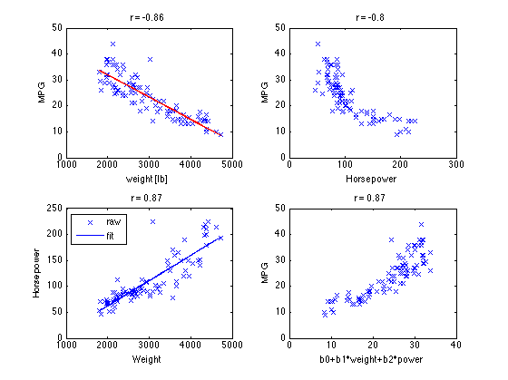
Read in small car dataset and plot mpg vs. weight

load carsmall
whos
isdata = isfinite(MPG)&isfinite(Weight)&isfinite(Horsepower);
y = MPG(isdata);
x = Weight(isdata);
N = length(y)
clf
subplot(2,2,1)
plot(x,y,'x')
xlabel('weight [lb]')
ylabel('MPG')
hold on

  Name                Size            Bytes  Class     Attributes

  Acceleration      100x1               800  double              
  Cylinders         100x1               800  double              
  Displacement      100x1               800  double              
  Horsepower        100x1               800  double              
  MPG               100x1               800  double              
  Mfg               100x13             2600  char                
  Model             100x33             6600  char                
  Model_Year        100x1               800  double              
  Origin            100x7              1400  char                
  Weight            100x1               800  double              


N =

    93

Linear regression analysis

r = corrcoef(x,y) % Corr coeff is the off-diagonal (1,2) element
r = r(1,2)  % Sample regression coefficient

% Add to the scatterplot
title(['r = ' num2str(0.01*round(r*100))])
xbar = mean(x);
ybar = mean(y);
sigx = std(x);
sigy = std(y);
a1 = r*sigy/sigx   % Regression line slope

% Overplot regression line, adding means back in.

yfit = ybar + a1*(x - xbar);
plot(x,yfit,'k-')

r =

    1.0000   -0.8591
   -0.8591    1.0000


r =

   -0.8591


a1 =

   -0.0086

Use Matlab regress function

X = [x ones(N,1)]; % Add column of 1's to include constant term in regression
a = regress(y,X)   % = [a1; a0]
plot(x,X*a,'r-');  % This line perfectly overlays the previous fit line

a =

   -0.0086
   49.2383

Multiple regression using weight and horsepower as predictors

Note weight and horsepower are highly correlated, so the additional
predictive power is unclear.

x1 = x;  % weight
x2 = Horsepower(isdata);
r12 = corrcoef(x1,x2);
r12 = r12(1,2);   % Correlation of weight and horsepower
ry2 = corrcoef(y,x2);
ry2 = ry2(1,2);   % Correlation of MPG and horsepower
x2fit = mean(x2)+(x1-mean(x1))*r12*std(x2)/std(x1); %Fit x2 to x1

subplot(2,2,2)
plot(x2,y,'bx')
xlabel('Horsepower')
ylabel('MPG')
title(['r = ' num2str(0.01*round(ry2*100))])

subplot(2,2,3)
plot(x1,x2,'bx',x1,x2fit,'b-')
legend('raw','fit','Location','NorthWest')
xlabel('Weight')
ylabel('Horsepower')
title(['r = ' num2str(0.01*round(r12*100))])


X = [x1 x2 ones(N,1)];
b = regress(y,X)
ry12 = corrcoef(y,X*b);
ry12 = ry12(1,2);
subplot(2,2,4)
plot(X*b,y,'x');
xlabel('b0+b1*weight+b2*power')
ylabel('MPG')
title(['r = ' num2str(0.01*round(ry12*100))])

b =

   -0.0066
   -0.0420
   47.7694

Stepwise regression

% Manually remove linear fit of y, x2 to predictor x1
x2tilde = x2 - x2fit;
ytilde = y - yfit;

% Now try linear regression of residual ytilde on x2tilde.
% If the |correlation coeff| is statistically significant (>2/sqrt(N)),
% we should keep the second predictor.

ry2t = corrcoef(ytilde,x2tilde);
ry2t = ry2t(1,2)

% Using Matlab
stepwisefit([x1 x2],y) % Shows x2 adds significantly to fit quality

ry2t =

   -0.2308

Initial columns included: none
Step 1, added column 1, p=3.24054e-28
Step 2, added column 2, p=0.02686
Final columns included:  1 2 
    'Coeff'      'Std.Err.'    'Status'    'P'         
    [-0.0066]    [  0.0011]    'In'        [1.3519e-08]
    [-0.0420]    [  0.0187]    'In'        [    0.0269]


ans =

   -0.0066
   -0.0420

Published with MATLAB® R2012b